PyTorch中RNN相关学习笔记

---

前言

一周多前打算从Tensorflow转PyTorch，感觉神经网络中RNN相关的一系列概念算是最复杂的了，需要沉下心来好好学学！

---

Torch.nn.RNN

官方API文档

描述

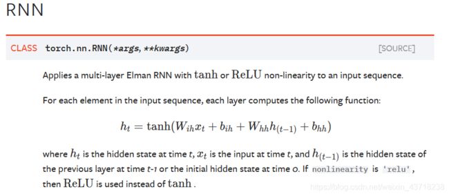
实现以$tanh$或$ReLU$为激活函数的多层RNN，PyTorch里$h_t$为所谓的隐藏状态（hidden state），其实是我认知中的${\mathbf{a}}^{<\mathbf{t}>}$, activation value。则上式即
$${\mathbf{a}}^{<\mathbf{t}>}=g({\mathbf{W}}_{\mathbf{a}}[{\mathbf{a}}^{<\mathbf{t}-1>},{\mathbf{x}}^{<\mathbf{t}>}]+{\mathbf{b}}_{\mathbf{a}})$$

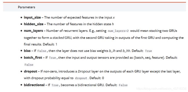
参数

input_size：输入x的维度（即特征features空间对应的维度）
hidden_size：隐藏状态的维度
num_layers：堆叠层数，默认为一层。
nonlinearity：非线性激活函数，默认tanh，可选relu。
bias：若为False则无bias
batch_first：若为True，则输入输出Shape为（batch_size，time_step, input_size）,默认为False，就是说我们的输入输出要尽量保持为(time_step, batch_size, input_size)， 然而常用的Shape其实是batch_size在前，这就需要我们在输入RNN前做permute
dropout：随机失活概率，若有值则给除了最后一层的所有层加上dropout层；默认为0。
bidirectional：若为True，则为双向RNN。使用双向RNN时，隐藏状态的维数应该需要变化。

输入输出

输入：
input：Shape为（time_step, batch_size, input_size），其中input_size即features，指的是每个时间步上的特征维度。
h_0：Shape为（num_layers * num_directions, batch_size, hidden_size）,每个batch的初始状态（${\mathbf{a}}^{<0>}$）,默认初始状态为0。num_directions只有1和2，2为双向RNN的情况。
输出：
output：Shape为（time_step, batch_size, num_directions * hidden_size）。这里的output是RNN最后一层 （不是最后一个时间步） 计算的隐藏状态$h^{[l]}$(即${\mathbf{a}}^{[\mathbf{l}]}$)，也就是说输出$y$需要
$$\mathbf{y}=g({\mathbf{W}}_{\mathbf{y}\mathbf{a}}{\mathbf{a}}^{[\mathbf{l}]}+{\mathbf{b}}_{\mathbf{y}})=g(\mathbf{W}\ast \mathbf{o}\mathbf{u}\mathbf{t}\mathbf{p}\mathbf{u}\mathbf{t}+{\mathbf{b}}_{\mathbf{y}})$$
使用双向RNN时，可以output.view(time_step, batch_size, num_directions, hidden_size)来把forward（[0]）和backward([1])分开。
h_n：Shape为（num_layers * num_directions, batch_size, hidden_size），最后一个时间步的隐藏状态${\mathbf{a}}^{<\mathbf{t}>}$, 同样可以由h_n.view(num_layers, num_directions, batch_size, hidden_size) 将双向RNN的前向和后向分开。

输入输出形状及变量

输入输出形状需要注意的是Input2（h_0, initial hidden state）的最后一个维度hidden size决定了输出的最后一个维度,即最后一层隐藏状态output1的最后一个维度为num_directions * hidden size, 最后一个时间步隐藏状态output2（h_n）的最后一个维度就是输入的初始状态h_0的最后一个维度hidden size。
生成变量：

RNN.weight_ih_l[k] - $W_{ih}^{[k]}$, $x^{<t>}$前的矩阵(我的习惯是把相乘的元素放在下标后边，PyTorch里$i$指$input,h$是我习惯的$a$：$W_{ax}^{[l]}$)
RNN.weight_hh_l[k] - $W_{hh}^{[k]}$, $h^{<t>[k]}$前的矩阵($W_{aa}^{[l]}$)
RNN.bias_ih_l[k] - $b_{ih}^{[k]}$, 与$x^{<t>}$有关的bias部分($b_{ax}^{[l]}$)
RNN.bias_hh_l[k] - $b_{hh}^{[k]}$, 与 $h^{<t>[k]}$有关的bias部分($b_{aa}^{[l]}$)
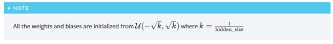注意：初始权重和偏置均为如上的均匀分布

小结

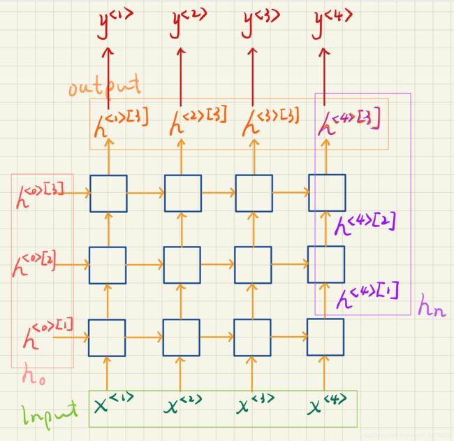
PyTorch中的input, h_0, output, h_n如下示意图所示，另外PyTorch中第一层是$l_0$。由图中可看出output[-1] 应该是要等于h_n[-1]的（在没有双向RNN的情况下），这将在代码部分验证

Coding Examples

上代码是比较重要的，嗯…不然就只是官方文档的翻译了…阅读文档只是为了辅助科研中的使用，毕竟RNN里边儿乱七八糟的东西太多了感觉。

import torch
import torch.nn.functional as F

简单RNN

验证形状是否正确

# input_size=hidden_size=1, layers=1
rnn = torch.nn.RNN(1, 1, nonlinearity='relu')
# time_step=16, batch_size=20, features=1
inputs = torch.ones([16, 20, 1])
# num_layers * num_directions = 1 * 1 = 1
h_0 = torch.zeros([1, 20, 1])

output, h_n = rnn(inputs, h_0)
# output shape: (time_step=16, batch_size=20, 1 * hidden_size = 1 * 1 = 1)
# h_n shape: (num_layer * num_directions = 1, batch_size = 20, hidden_size = 1)
# Validation:
print('output.shape: \t', output.shape)
print('h_n.shape: \t', h_n.shape)

输出结果：

与推测相符~
接下来检验内部运算，为避免偶然，将输入改为高斯分布：

# time_step=16, batch_size=20, features=1
inputs = torch.randn([16, 20, 1])
# num_layers * num_directions = 1 * 1 = 1
h_0 = torch.randn([1, 20, 1])

验证下式:
$$h_t=ReLU(W_{ih}{x}_t+b_{ih}+W_{hh}{h}_{(t-1)}+b_{hh})$$
对于output[0]，它是第一个时间步上所有batch_size的最后一层隐藏状态（$h^{<t>[l]}$），这里我们只有一层，所以只进行一次计算:

w_ih = rnn.weight_ih_l0
w_hh = rnn.weight_hh_l0
b_ih = rnn.bias_ih_l0
b_hh = rnn.bias_hh_l0
print('rnn.weight_ih_l0: \t', w_ih)
print('rnn.weight_hh_l0: \t', w_hh)
print('rnn.bias_ih_l0: \t', b_ih)
print('rnn.bias_hh_l0: \t', b_hh)

h_1 = F.relu(w_ih * inputs[0] + b_ih + w_hh * h_0[0] + b_hh)
print('h_1: \n', h_1)
assert all(h_1[i] == output[0][i] for i in range(20))

接下来验证output[-1] 是否等于h_n[-1]，注意这里的20和上面的20都是batch_size：

assert all(output[-1][i] == h_n[-1][i] for i in range(20))

双向RNN

INPUT_SIZE = 10
HIDDEN_SIZE = 20
NUM_LAYERS = 4
BATCH_SIZE = 5
TIME_STEP = 16

bi_rnn = torch.nn.RNN(INPUT_SIZE, HIDDEN_SIZE, NUM_LAYERS, nonlinearity='relu', bidirectional=True, bias=False)
inputs = torch.randn(TIME_STEP, BATCH_SIZE, INPUT_SIZE)
# Here num_directions = 2 since we are using bidirectional RNN:
h_0 = torch.randn(2 * NUM_LAYERS, BATCH_SIZE, HIDDEN_SIZE)

output, h_n = bi_rnn(inputs, h_0)
# Output should be in shape of (TIME_STEP, BATCH_SIZE, 2 * HIDDEN_SIZE)
# H_n should be in shape of (2 * NUM_LAYERS, BATCH_SIZE, HIDDEN_SIZE)

验证形状

# Validation:
assert output.shape[0] == TIME_STEP
assert output.shape[1] == BATCH_SIZE
assert output.shape[2] == 2 * HIDDEN_SIZE
assert h_n.shape[0] == 2 * NUM_LAYERS
assert h_n.shape[1] == BATCH_SIZE
assert h_n.shape[2] == HIDDEN_SIZE

实际上，在经典RNN中，最终输出${\mathbf{y}}^{<\mathbf{l}>}=g({\mathbf{W}}_{\mathbf{y}\mathbf{a}}{\mathbf{a}}^{<\mathbf{l}>}+{\mathbf{b}}_{\mathbf{y}})$, 因此我们还需要对rnn的输出做一次矩阵相乘并通过一个激活函数。且由于当前RNN为双向，我们还需要把forward和backward提取出来，并拼接在一起进而得到最终输出：
$${\mathbf{y}}^{<\mathbf{t}>}=g(W_{ya}[{\mathbf{a}}^{<\mathbf{t}>},{\mathbf{a}}^{<\mathbf{t}>}]+{\mathbf{b}}_{\mathbf{y}})$$
这里单个方向上的隐藏状态形状原本为([16, 5, 20]),拼接后将变为([16, 5, 40])：

# Separate the directions
output_reshape = output.view(TIME_STEP, BATCH_SIZE, -1, HIDDEN_SIZE)
# concatenate the both directions
output_cat = torch.cat([output_reshape[:, :, 0, :], output_reshape[:, :, 1, :]], dim=-1)

我们想要的输出$y$的形状应该是([16, 5, 20]),于是这里创建形状为([20, 40])的权重和形状为([20])的偏置，与拼接后的隐藏状态相乘后通过一个$tanh$函数，得到最终输出y：

# weight_yh (hidden_size, 2 * hidden_size)
# bias_y (hidden_size)
w_yh = torch.randn([HIDDEN_SIZE, output.shape[2]])
b_y = torch.randn(HIDDEN_SIZE)
# (time_step, batch_size, 2 * hidden_size) * (2 * hidden_size, hidden_size)
y = torch.tanh(torch.matmul(output_cat, w_yh.T) + b_y)

y的形状是正确的：

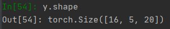
接下来检查output的最后一个时间步是否等于h_n的最后一层。由于这里是双向RNN，把h_n按方向分开之后，对于forward的部分，应该有output[-1] == h_n[-1]，而对于backward部分，output应该是反过来的，即output[0] == h_n[-1],因为backward output的第一个时间步就是相对于整个RNN来说的最后一个时间步。

# check the last time step of forward direction and the first time step of backward direction
h_n_reshape = h_n.view(NUM_LAYERS, -1, BATCH_SIZE, HIDDEN_SIZE)
assert (h_n_reshape[-1, 0, :, :] == output_reshape[-1, :, 0, :]).all()
assert (h_n_reshape[-1, 1, :, :] == output_reshape[0, :, 1, :]).all()

至此，最简单的RNN和双向RNN应该熟悉一些了~

Torch.nn.GRU 和 Torch.nn.LSTM

写着写着发现GRU和RNN的API真的很相似，所以把LSTM放到和GRU一起说，LSTM 加入的变化会多一些

GRU官方文档

描述

$r_t$为重置门（${\Gamma }_r^{<t>}$)，$z_t$为更新门（${\Gamma }_u^{<t>}$）,$n_t$这里叫做new gate，其实就是我理解的candidate cell （${\tilde{h}}^{<t>}$ or ${\tilde{c}}^{<t>}$）。需要注意的是$n_t$的计算中重置门$r_t$与前一个隐藏状态$h_{(t-1)}$部分的乘积是Hadamard积，即entity-wise的对应元素相乘。其他的表示和前面的RNN相似。

参数、输入输出及形状

参数：
和RNN的一样，只是没有提供nonlinearity来选择激活函数，好！
看了一下输入输出和形状都和RNN一样，这里也就不截图了前面的RNN熟悉之后后面的轻松很多~

变量

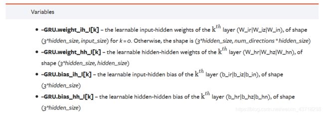这里的weight_ih指与输入x相乘的权重，因为涉及到两个门（reset gate,${\Gamma }_r^{<t>}$ and update gate, ${\Gamma }_u^{<t>}$）和一个candidate cell（${\tilde{h}}^{<t>}$ or ${\tilde{c}}^{<t>}$）,所以其形状涉及到hidden_size 的要乘以3；与hidden state相乘的weight_hh、以及两个偏置bias_ih和bias_hh也是如此。
权重和偏置同样也是以均匀分布进行初始化。

LSTM官方文档

描述

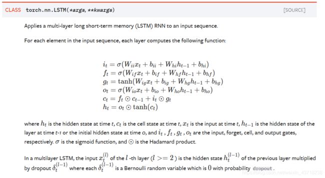第一眼看这个的时候…什么乱七八糟的，好好起名字会死吗…不管文档里怎么定义了，我只要我觉得…
全部按我的来替换掉：
$i_t$ (update gate, ${\Gamma }_u^{<t>}$) , $f_t$ (forget gate, ${\Gamma }_f^{<t>}$), $g_t$ (candidate cell, ${\tilde{c}}^{<t>}$),
$o_t$ (output gate, ${\Gamma }_o^{<t>}$), $c_t$ (memory cell), $h_t$ (hidden state, or activation value)
那和三个门相关的更新公式就是：
$$c_t={\Gamma }_f^{<t>}\odot c_{t-1}+{\Gamma }_u^{<t>}\odot {\tilde{c}}^{<t>}$$
$$h_t={\Gamma }_o^{<t>}\odot tanh(c_t)$$

输入输出

参数和GRU的一样就不提了，看输入输出：
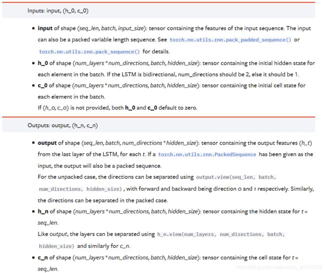好家伙，多了个c_0和c_n，所有和$c$有关的都是memory cell记忆单元相关部分。事实上$c$和$h$因为保持着对应的关系（entity-wise product）所以有相同的形状，把这点牢记在心对LSTM的运用应该也不难把握了。
candidate cell(${\tilde{c}}^{<t>}$)是接口内部运算才会涉及到的变量，不考虑它的话，其实也就只有$c^{<t>}$和$h^{<t>}$需要我们斟酌了。然而$h^{<t>}$是输出门${\Gamma }_o^{<t>}$和经过$tanh$之后的$c^{<t>}$通过对应元素相乘得到的，它们自然也应该有相同的shape~
另外小细节就是这里的输入h_0和c_0要以一个元组cell输入，即(h_0, c_0)，输出也是以元组的形式输出的：(h_n, c_n)；如果没注意到等报错了TypeError: forward() takes from 2 to 3 positional arguments but 4 were given就会注意到了…

变量

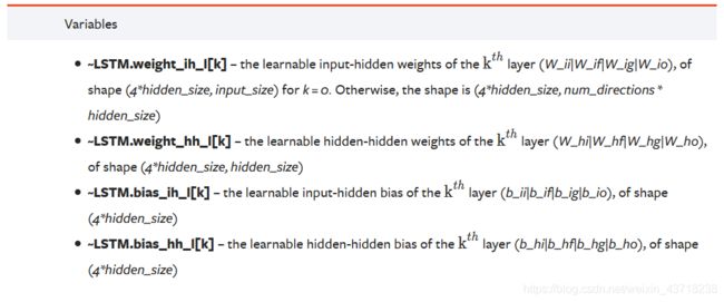
PyTorch里把candidate cell也叫做一个门：cell gate（单元门？？），这样的话一个LSTM类里其实有四个门，那对应的权重和偏置相应的形状要乘以4。权重的初始化也和GRU一样。
当然啦我还是不习惯把candidate cell看作一个gate，因为它显然起的不是一个门的作用，而是新的记忆单元memory cell的候选项。

Coding Examples

GRU 和 LSTM 其实和前面的RNN在接口的使用上没有什么太大不同，不过是LSTM会多了一个memory cell而已，那我就只放一个LSTM的简单使用好了~
参数和之前的一样：

INPUT_SIZE = 10
HIDDEN_SIZE = 20
NUM_LAYERS = 4
BATCH_SIZE = 5
TIME_STEP = 16

简单的实现：

lstm = torch.nn.LSTM(INPUT_SIZE, HIDDEN_SIZE, NUM_LAYERS, bias=False)
inputs = torch.randn(TIME_STEP, BATCH_SIZE, INPUT_SIZE)
h_0 = torch.randn(NUM_LAYERS, BATCH_SIZE, HIDDEN_SIZE)
c_0 = torch.randn(NUM_LAYERS, BATCH_SIZE, HIDDEN_SIZE)

outputs, (h_n, c_n) = lstm(inputs, (h_0, c_0))

还有一个更简单的：

outputs, (h_n, c_n) = lstm(inputs)

如果接受$h$和$c$的初始值都是0的话完全可以不输入h_0和c_0~

拜拜语

有前言要有结语，到这里为止其实还只是开始。
祝大家学业有成，新年快乐~
（看论文去了…)