cp12_实现a M ArtificialNN_gzip_mnist_struct_savez_compressed_fetch_openml_back propagation_weight更_L2
As you may know, deep learning is getting a lot of attention from the press and is without any doubt the hottest topic in the machine learning field. Deep learning can be understood as a subfield of machine learning that is concerned with training artificial neural networks (NNs) with many layers efficiently. In this chapter, you will learn the basic concepts of artificial NNs so that you are well equipped for the following chapters, which will introduce advanced Python-based deep learning libraries and deep neural network (DNN) architectures that are particularly well suited for image and text analyses.
The topics that we will cover in this chapter are as follows:
- • Gaining a conceptual understanding of multilayer NNs
- • Implementing the fundamental backpropagation algorithm for NN training from scratch
- • Training a basic multilayer NN for image classification
Modeling complex functions with artificial neural networks
At the beginning of this book, we started our journey through machine learning algorithms with artificial neurons in cp2_Training Simple Machine Learning Algorithms For Classification_meshgrid_ravel_contourf_OvA_Gradient Descent https://blog.csdn.net/Linli522362242/article/details/96429442. Artificial neurons represent the building blocks of the multilayer artificial NNs that we will discuss in this chapter.
However, in the decades that followed the first implementation of the McCulloch-Pitts neuron model—Rosenblatt's perceptron in the 1950s — many researchers and machine learning practitioners slowly began to lose interest in NNs since no one had a good solution for training an NN with multiple layers. Eventually, interest in NNs was rekindled in 1986 when D.E. Rumelhart, G.E. Hinton, and R.J. Williams were involved in the (re)discovery and popularization of the backpropagation algorithm to train NNs more efficiently, which we will discuss in more detail later in this chapter (Learning representations by back-propagating errors, D. E. Rumelhart, G. E. Hinton, R. J. Williams, Nature, 323 (6088): 533–536, 1986). Readers who are interested in the history of artificial intelligence (AI), machine learning, and NNs are also encouraged to read the Wikipedia article on the so-called AI winters, which are the periods of time where a large portion of the research community lost interest in the study of NNs (https://en.wikipedia.org/wiki/AI_winter).
However, NNs are more popular today than ever thanks to the many major breakthroughs that have been made in the previous decade, which resulted in what we now call deep learning algorithms and architectures—NNs that are composed of many layers. NNs are a hot topic not only in academic research but also in big technology companies, such as Facebook, Microsoft, Amazon, Uber, and Google, that invest heavily in artificial NNs and deep learning research.
As of today, complex NNs powered by deep learning algorithms are considered the state-of-the-art solutions最前沿的研究成果 for complex problem solving such as image and voice recognition. Popular examples of the products in our everyday life that are powered by deep learning are Google's image search and Google Translate—an application for smartphones that can automatically recognize text in images for real-time translation into more than 20 languages.
Many exciting applications of DNNs have been developed at major tech companies and the pharmaceutical[ˌfɑːrməˈsuːtɪkl]制药的 industry as listed in the following, non-comprehensive list of examples:
- Facebook's DeepFace for tagging images (DeepFace: Closing the Gap to Human-Level Performance in Face Verification, Y. Taigman, M. Yang, M. Ranzato, and L. Wolf, IEEE Conference on Computer Vision and Pattern Recognition (CVPR), pages 1701–1708, 2014)
- Baidu's DeepSpeech, which is able to handle voice queries in Mandarin (DeepSpeech: Scaling up end-to-end speech recognition, A. Hannun, C. Case, J.Casper, B. Catanzaro, G. Diamos, E. Elsen, R. Prenger, S. Satheesh, S. Sengupta, A. Coates, and Andrew Y. Ng, arXiv preprint arXiv:1412.5567, 2014)
- Google's new language translation service (Google's Neural Machine Translation System: Bridging the Gap between Human and Machine Translation, arXiv preprint arXiv:1412.5567, 2016)
- Novel techniques for drug discovery and toxicity[tɑkˈsɪsəti]毒性prediction (Toxicity prediction using Deep Learning, T. Unterthiner, A. Mayr, G. Klambauer, and S. Hochreiter, arXiv preprint arXiv:1503.01445, 2015)
- A mobile application that can detect skin cancer with an accuracy similar to professionally trained dermatologists[ˌdə:məˈtɔlədʒists]皮肤病学家(Dermatologist-level classification of skin cancer with deep neural networks, A. Esteva, B.Kuprel, R. A. Novoa, J. Ko, S. M. Swetter, H. M. Blau, and S.Thrun, in Nature 542, no. 7639, 2017, pages 115-118)
- Protein 3D structure prediction from gene sequences (De novo structure prediction with deep-learning based scoring, R. Evans, J. Jumper, J. Kirkpatrick, L. Sifre, T.F.G. Green, C. Qin, A. Zidek, A. Nelson, A. Bridgland, H. Penedones, S. Petersen, K. Simonyan, S. Crossan, D.T. Jones, D. Silver, K. Kavukcuoglu, D. Hassabis, and A.W. Senior, in Thirteenth Critical Assessment of Techniques for Protein Structure Prediction, 1-4 December, 2018)
- Learning how to drive in dense traffic from purely observational data such as camera video streams (Model-predictive policy learning with uncertainty regularization for driving in dense traffic, M. Henaff, A. Canziani, Y. LeCun, 2019, in Conference Proceedings of the International Conference on Learning Representations, ICLR, 2019)
Single-layer neural network recap
This chapter is all about multilayer NNs, how they work, and how to train them to solve complex problems. However, before we dig deeper into a particular multilayer NN architecture, let's briefly reiterate some of the concepts of single-layer NNs that we introduced in cp2_Training Simple Machine Learning Algorithms For Classification_meshgrid_ravel_contourf_OvA_Gradient Descent https://blog.csdn.net/Linli522362242/article/details/96429442, namely, the ADAptive LInear NEuron (Adaline) algorithm, which is shown in the following figure: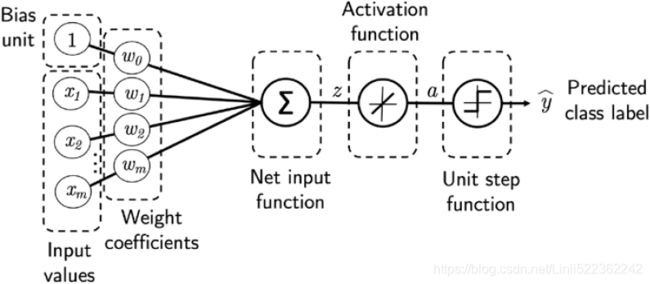
import numpy as np
class AdalineGD(object):
#Parameters
# eta: Learning rate (between 0.0 and 1.0)
# n_iter: Passes over the training dataset
# random_state: Random number generator seed for random weight
#Attributes
# w_ : 1d-array # weights after fitting
# cost_ : Sum-of-squares cost function value in each epoch
#random seed
def __init__(self, eta=0.01, n_iter=50, random_state=1):
self.eta = eta
self.n_iter = n_iter
self.random_state = random_state
def net_input(self, X): #intercept
return np.dot(X, self.w_[1:]) + self.w_[0] # X(samples, features) dot w(1+features,1) ==> a single column matrix
def activation(self, X):
#Computer linear activation
return X
def fit(self, X, y): #X_array = [n_samples, n_features]
#y: label =[n_samples]
rgen = np.random.RandomState(self.random_state) #1+ n_features
self.w_ = rgen.normal( loc=0.0, scale=0.01, size=1+X.shape[1] )
self.cost_ = []
for i in range(self.n_iter):
net_input = self.net_input(X) # single column matrix
output = self.activation(net_input) #single column matrix
errors = (y-output) # result_vertical #single column matrix #rows == number of X_samples
#feature_weight
self.w_[1:] += self.eta * X.T.dot(errors) # X.T (n_features, n_samples) #single column matrix#rows==numberOfFeatures
self.w_[0] += self.eta * errors.sum()
cost = (errors **2).sum() /2.0
self.cost_.append(cost)
return self # update weights and minimize cost function
def predict(self, X):
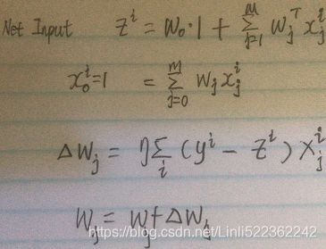
return np.where( self.activation( self.net_input(X) )>=0.0, 1, -1 )In cp2_Training Simple Machine Learning Algorithms For Classification_meshgrid_ravel_contourf_OvA_Gradient Descent https://blog.csdn.net/Linli522362242/article/details/96429442, we implemented the Adaline algorithm to perform binary classification, and we used the gradient descent optimization algorithm to learn the weight coefficients of the model. In every epoch (pass over the training dataset), we updated the weight vector w using the following update rule:
![]() and
and 
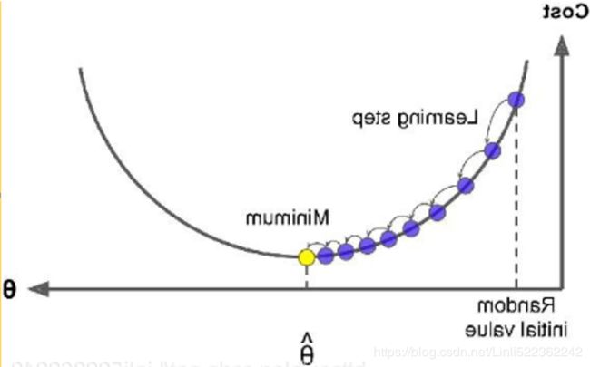
In other words, we computed the gradient based on the whole training dataset and updated the weights of the model by taking a step into the opposite direction of the gradient ∇J() . In order to find the optimal weights of the model, we optimized an objective function that we defined as the sum of squared errors (SSE) cost function J() . Furthermore, we multiplied the gradient by a factor, the learning rate , which we had to choose carefully to balance the speed of learning against the risk of overshooting the global minimum of the cost function.
In gradient descent optimization, we updated all weights simultaneously after each epoch, and we defined the partial derivative for each weight ![]() in the weight vector w as follows:
in the weight vector w as follows: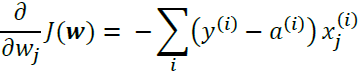 OR
OR 
Here, ![]() is the target class label of a particular sample
is the target class label of a particular sample ![]() , and
, and ![]() is the activation of the neuron, which is a linear function in the special case of Adaline.
is the activation of the neuron, which is a linear function in the special case of Adaline.
Furthermore, we defined the activation function (∙) as follows: ![]()
Here, the net input, z, is a linear combination of the weights that are connecting the input layer to the output layer: 
While we used the activation () to compute the gradient update, we implemented a threshold function(a unit step function) to squash the continuous valued output into binary class labels for prediction: 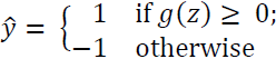
#########################################################
Single-layer naming convention
Note that although Adaline consists of two layers, one input layer and one output layer, it is called a single-layer network because of its single link between the input and output layers.
#########################################################
Also, we learned about a certain trick to accelerate the model learning, the so-called stochastic gradient descent (SGD, update the weights incrementally for each training sample:  To obtain satisfying results via stochastic gradient descent, it is important to present it training data in a random order; also, we want to shuffle the training set for every epoch to prevent cycles. In stochastic gradient descent implementations, the fixed learning rate
 ![]() is often replaced by an adaptive learning rate that decreases over time, for example,
is often replaced by an adaptive learning rate that decreases over time, for example,  where
where ![]() and
and ![]() are constants. Note that stochastic gradient descent does not reach the global minimum but an area very close to it.
are constants. Note that stochastic gradient descent does not reach the global minimum but an area very close to it.

class AdalineSGD(object):
    #Parameters
    # eta: Learning rate (between 0.0 and 1.0)
    # n_iter: Passes over the training dataset
    # shuffle : bool (default: True) Shuffles training data every epoch if True to prevent cycles.
    # random_state: Random number generator seed for random weight

    #Attributes
    # w_ : 1d-array # weights after fitting
    # cost_ : Sum-of-squares cost function value in each epoch
                                            #random seed
    def __init__(self, eta=0.01, n_iter=10, shuffle=True, random_state=None):
        self.eta = eta
        self.n_iter = n_iter
        self.w_initialized = False#############
        self.shuffle = shuffle#############
        self.random_state=random_state

    def _initialize_weights(self, m):
        self.rgen = np.random.RandomState(self.random_state)
        self.w_ = self.rgen.normal(loc=0.0, scale=0.01, size=1+m) #numOfFeatures + 1
        self.w_initialized = True

    def activation(self, X):
        return X

    def net_input(self, X):
        return np.dot(X, self.w_[1:]) + self.w_[0]

    def _shuffle(self, X,y):
        r=self.rgen.permutation(len(y)) #shuffle
        return X[r], y[r] #selection or pick in order(r)

    def _update_weights(self, xi, target):
        # Apply Adaline learning rule to update the weights
        output = self.activation( self.net_input(xi) )
        error = (target - output)
        # VS self.w_[1:] += self.eta * X.T.dot(errors) # X.T (n_features, n_samples)
        self.w_[1:] += self.eta * xi.dot(error) ### update the weights for "each sample"###

        self.w_[0] += self.eta * error
        cost = 0.5 * error**2
        return cost # update the weights for "each sample" and compute cost for "each sample"

    def fit(self, X, y): # X : {array-like}, shape = [n_samples, n_features]
        self._initialize_weights(X.shape[1]) ### step 1 ###
        self.cost_ = []
        for i in range(self.n_iter):         ### step 2 ###
            if self.shuffle:
                X, y = self._shuffle(X,y)
            cost = []
            for xi, target in zip(X,y):
                cost.append(self._update_weights(xi, target)) #append all costs of samples

            avg_cost = sum(cost) / len(y)
            self.cost_.append(avg_cost)
        return self

    def partial_fit(self, X, y):
        if not self.w_initialized: #has not reinitialize the weights
            self._initialize_weights(X.shape[1]) # X.shape[1]== number of features

        if y.ravel().shape[0] > 1:
            for xi, target in zip(X,y):
                self._update_weights(xi, target)
        else:
            self._update_weights(X,y)
        return self

    def predict(self, X):
        return np.where(self.activation(self.net_input(X))>=0.0, 1, -1
The _shuffle method that we are now using in the AdalineSGD classifier works as follows: via the permutation function in np.random, we generate a random sequence of unique numbers in the range 0 to 100. Those numbers can then be used as indices to shuffle our feature matrix and class label vector. https://blog.csdn.net/Linli522362242/article/details/96429442
#OR
This code implements Stochastic Gradient Descent using a simple learning schedule:
X = 2*np.random.rand(100,1) # 100rows 1column
   #4:intercept 3:weigtht # random error
y = 4 + 3*X + np.random.randn(100,1)
X_b = np.c_[np.ones( (100,1) ), X] #add x0=1 to each instance, X0==1
theta_path_sgd = []
m=len(X_b) #=X_b.shape[0]
np.random.seed(42)

n_epochs = 50
t0,t1= 5,50

def learning_schedule(t):
    return t0/(t+t1)

theta = np.random.randn(2,1)

for epoch in range(n_epochs): # n_epochs=50 replaces n_iterations=1000
    for i in range(m): # m = len(X_b)
        if epoch==0 and i<20:
            y_predict = X_new_b.dot(theta)
            style="b-" if i>0 else "r--"
            plt.plot(X_new,y_predict, style)######

        random_index = np.random.randint(m)  ##### Stochastic
        xi = X_b[random_index:random_index+1]
        yi = y[random_index:random_index+1]
        gradients = 2*xi.T.dot( xi.dot(theta) - yi ) ##### Gradient
        eta=learning_schedule(epoch*m + i) ############## e.g. 5/( (epoch*m+i)+50)
        theta = theta-eta * gradients  ###### Descent
        theta_path_sgd.append(theta)


plt.plot(X, y, "b.")
plt.xlabel("$x_1$", fontsize=18)
plt.ylabel("$y$", rotation=0, fontsize=18)
plt.title("Figure 4-10. Stochastic Gradient Descent first 10 steps")

plt.axis([0,2, 0,15])

####################################################### https://blog.csdn.net/Linli522362242/article/details/104005906
Batch Gradient Descent
Equation 4-5 computes the partial derivative of the cost function with regards to parameter  (OR weight wj), noted
 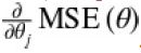 .
.
Note:cost function 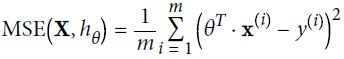 # m is the number of samples (or batch size is m)
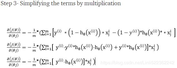
Equation 4-5. Partial derivatives of the cost function(start with  or i >=1) ### j is the index on Weight coefficient term w_j (OR the index j of feature coefficient term)
 ==
== * 2 (without adding the term
  to the calculation process.)
Instead of computing these gradients individually(), you can use Equation 4-6 to compute them all in one go. The gradient vector, noted 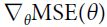 , contains all the partial derivatives of the cost function (one for each model parameter, or weight wj).
Equation 4-1. Linear Regression model prediction (X0==1, X0 *  ==, the bias term also is w0 )

Equation 4-6. Gradient vector of the cost function ( for equation 4-5)
 Note:
Note:  ==
==  *2
*2
(without adding the term to the calculation process.)
Once you have the gradient vector, which points uphill, just go in the opposite direction to go downhill. This means subtracting 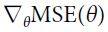 from θ. This is where the learning rate η( η reads Eta, or
  )comes into play: multiply the gradient vector by η to determine the size of the downhill step (Equation 4-7).
Equation 4-7. Gradient Descent step 
X = 2*np.random.rand(100,1) # 100rows 1column
 #4:intercept 3:weigtht # random error
y = 4 + 3*X + np.random.randn(100,1)
X_b = np.c_[np.ones( (100,1) ), X] #add x0=1 to each instance, X0==1

eta = 0.1 # learning rate
n_iterations = 1000
m=100

theta = np.random.randn(2,1) # random initialization

for iteration in range(n_iterations):
    gradients = 2/m * X_b.T.dot( X_b.dot(theta) - y )
    theta = theta - eta*gradients

theta #lin_reg.intercept_, lin_reg.coef_  #theta_best
X_new_b.dot(theta) #predictions
#######################################################
By using an adaptive learning rate, we can achieve further annealing磨炼 to a better global minimum) optimization. SGD approximates the cost from a single training sample (online learning) or a small subset of training examples (mini-batch learning, A compromise between batch gradient descent and stochastic gradient descent is socalled mini-batch learning. Mini-batch learning can be understood as applying batch gradient descent to smaller subsets of the training data, for example, 32 samples at a time. The advantage over batch gradient descent is that convergence is reached faster via mini-batches because of the more frequent weight updates. Furthermore, mini-batch learning allows us to replace the for loop over the training samples in stochastic gradient descent with vectorized operations, which can further improve the computational efficiency of our learning algorithm.).
#######################################################https://blog.csdn.net/Linli522362242/article/details/104005906
a simple learning schedule:
X = 2*np.random.rand(100,1) # 100rows 1column
 #4:intercept 3:weigtht # random error
y = 4 + 3*X + np.random.randn(100,1)
X_b = np.c_[np.ones( (100,1) ), X] #add x0=1 to each instance, X0==1

theta_path_mgd = []

n_iterations = 50
minibatch_size=20

np.random.seed(42)
theta = np.random.randn(2,1) # Normal Distribution(0,1)=(u,sigma)

t0, t1 =200, 1000
def learning_schedule(t):
    return t0/(t+t1)

t=0
for epoch in range(n_iterations):
    shuffled_indices = np.random.permutation(m)
    X_b_shuffled = X_b[shuffled_indices]
    y_shuffled = y[shuffled_indices]
    for i in range(0,m, minibatch_size):########
        t += 1
        xi = X_b_shuffled[i:i+minibatch_size]
        yi = y_shuffled[i:i+minibatch_size]
        gradients = 2/minibatch_size * xi.T.dot( xi.dot(theta)-yi)
        eta = learning_schedule(t)
        theta = theta-eta*gradients
        theta_path_mgd.append(theta)

theta
theta_path_bgd = np.array(theta_path_bgd)
theta_path_sgd = np.array(theta_path_sgd)
theta_path_mgd = np.array(theta_path_mgd)

plt.figure( figsize=(7,4) )
plt.plot(theta_path_sgd[:,0], theta_path_sgd[:,1], "y-s", linewidth=1, label="Stochastic")
plt.plot(theta_path_mgd[:,0], theta_path_mgd[:,1], "g-x", linewidth=1, label="Mini-batch" )
plt.plot(theta_path_bgd[:,0], theta_path_bgd[:,1], "b-o", linewidth=1, label="Batch")

plt.legend(loc="upper left", fontsize=16)
plt.xlabel(r"$\theta_0$", fontsize=20)
plt.ylabel(r"$\theta_1$", fontsize=20, rotation=0)
plt.axis([2.5, 4.5, 2.3, 3.9])
plt.title("Figure 4-11. Gradient Descent paths in parameter space")
plt.show()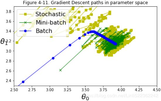
The (Mini-batch Gradient Descent's) algorithm’s progress in parameter space is less erratic不规则的 than with SGD(Stocastic Gradient Descent), especially with fairly large mini-batches(Batch). As a result, Mini-batch GD will end up walking around a bit closer to the minimum than SGD. But, on the other hand, it may be harder for it to escape from local minima (in the case of problems that suffer from local minima, unlike Linear Regression as we saw earlier). Figure 4-11 shows the paths taken by the three Gradient Descent algorithms in parameter space during training. They all end up near the minimum, but Batch GD’s path actually stops at the minimum, while both Stochastic GD and Mini-batch GD continue to walk around. However, don’t forget that Batch GD takes a lot of time to take each step, and Stochastic GD and Mini-batch GD would also reach the minimum if you used a good learning schedule.
#######################################################
We will make use of this concept later in this chapter when we implement and train a multilayer perceptron (MLP). Apart from faster learning—due to the more frequent weight updates compared to gradient descent—its noisy nature is also regarded as beneficial when training multilayer NNs with nonlinear activation functions, which do not have a convex cost function. Here, the added noise can help to escape local cost minima, but we will discuss this topic in more detail later in this chapter.
Introducing the multilayer neural network architecture
In this section, you will learn how to connect multiple single neurons to a multilayer feedforward NN; this special type of fully connected network is also called MLP.
The following figure illustrates the concept of an MLP consisting of three layers: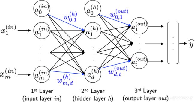
The MLP depicted in the preceding figure has one input layer, one hidden layer, and one output layer. The units in the hidden layer are fully connected to the input layer, and the output layer is fully connected to the hidden layer. If such a network has more than one hidden layer, we also call it a deep artificial NN.
Figure 10-6. XOR classification problem and an MLP that solves it https://blog.csdn.net/Linli522362242/article/details/106433059
##################################
Adding additional hidden layers
We can add any number of hidden layers to the MLP to create deeper network architectures. Practically, we can think of the number of layers and units in an NN as additional
hyperparameters that we want to optimize for a given problem task using cross-validation technique, which we discussed in cp6_Model Eval_Confusion_Hyperparameters Tuning_pipeline_variance_bias_ validation_learning curve_strength https://blog.csdn.net/Linli522362242/article/details/109560084.
However, the error gradients, which we will calculate later via backpropagation, will become increasingly small as more layers are added to a network. This vanishing gradient problem makes the model learning more challenging. Therefore, special algorithms have been developed to help train such DNN structures; this is known as deep learning.
##################################
As shown in the preceding figure, we denote the ith activation unit in the ith layer as ![]() . To make the math and code implementations a bit more intuitive, we will not use numerical indices to refer to layers, but we will use the in superscript for the input layer, the h superscript for the hidden layer, and the out superscript for the output layer. For instance,
. To make the math and code implementations a bit more intuitive, we will not use numerical indices to refer to layers, but we will use the in superscript for the input layer, the h superscript for the hidden layer, and the out superscript for the output layer. For instance, ![]() refers to the ith value in the input layer,
refers to the ith value in the input layer, ![]() refers to the ith unit in the hidden layer, and
refers to the ith unit in the hidden layer, and ![]() refers to the ith unit in the output layer. Here, the activation units
refers to the ith unit in the output layer. Here, the activation units ![]() and
and ![]() )are the bias units, which we set equal to 1. The activation of the units in the input layer is just its input plus the bias unit:
)are the bias units, which we set equal to 1. The activation of the units in the input layer is just its input plus the bias unit: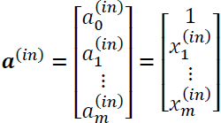
##################################
Notational convention for the bias units
Later in this chapter, we will implement an MLP using separate vectors for the bias units, which makes code implementation more efficient and easier to read. This concept is also used by TensorFlow, a deep learning library that we will cover in Chapter 13, Parallelizing Neural Network Training with TensorFlow. However, the mathematical equations that will follow would appear more complex or convoluted if we had to work with additional variables for the bias. Note that the computation via appending 1s to the input vector (as shown previously) and using a weight variable as bias is exactly the same as operating with separate bias vectors; it is merely a different convention.
##################################
Each unit in layer l is connected to all units in layer l + 1 via a weight coefficient. For example, the connection between the kth unit in layer l to the jth unit in layer l + 1 will be written as ![]() . Referring back to the previous figure, we denote the weight matrix that connects the input to the hidden layer as
. Referring back to the previous figure, we denote the weight matrix that connects the input to the hidden layer as ![]() , and we write the matrix that connects the hidden layer to the output layer as
, and we write the matrix that connects the hidden layer to the output layer as ![]() .
.
While one unit in the output layer would suffice for a binary classification task, we saw a more general form of NN in the preceding figure, which allows us to perform multiclass classification via a generalization of the one-versus-all (OvA) technique. To better understand how this works, remember the one-hot representation of categorical variables that we introduced in cp4 Training Sets Preprocessing_StringIO_dropna_categorical_feature_Encode_Scale_L1_L2_bbox_to_anchor https://blog.csdn.net/Linli522362242/article/details/108230328.
For example, we can encode the three class labels in the familiar Iris dataset (0=Setosa, 1=Versicolor, 2=Virginica) as follows:
This one-hot vector representation allows us to tackle classification tasks with an arbitrary number of unique class labels present in the training dataset.
If you are new to NN representations, the indexing notation (subscripts and superscripts) may look a little bit confusing at first. What may seem overly complicated at first will make much more sense in later sections when we vectorize the NN representation. As introduced earlier, we summarize the weights that connect the input and hidden layers by a matrix ![]() ∈
∈ ![]() , where d is the number of hidden units and m is the number of input units including the bias unit. Since it is important to internalize this notation to follow the concepts later in this chapter, let's summarize what we have just learned in a descriptive illustration of a simplified 3-4-3 MLP:
, where d is the number of hidden units and m is the number of input units including the bias unit. Since it is important to internalize this notation to follow the concepts later in this chapter, let's summarize what we have just learned in a descriptive illustration of a simplified 3-4-3 MLP: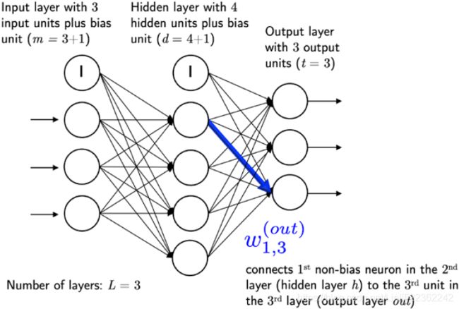
Activating a neural network via forward propagation
In this section, we will describe the process of forward propagation to calculate the output of an MLP model. To understand how it fits into the context of learning an MLP model, let's summarize the MLP learning procedure in three simple steps:
- 1. Starting at the input layer, we forward propagate the patterns of the training data through the network to generate an output.
- 2. Based on the network's output, we calculate the error that we want to minimize using a cost function that we will describe later.
- 3. We backpropagate the error, find its derivative with respect to each weight in the network, and update the model.
Finally, after we repeat these three steps for multiple epochs and learn the weights of the MLP, we use forward propagation to calculate the network output and apply a threshold function(a unit step function) to obtain the predicted class labels in the one-hot representation, which we described in the previous section.
Now, let's walk through the individual steps of forward propagation to generate an output from the patterns in the training data. Since each unit in the hidden layer is connected to all units in the input layers, we first calculate the activation unit of the hidden layer ![]() as follows:
as follows:
Here, ![]() is the net input and (∙) is the activation function, which has to be differentiable to learn the weights that connect the neurons using a gradient-based approach. To be able to solve complex problems such as image classification, we need nonlinear activation functions in our MLP model, for example, the sigmoid (logistic) activation function that we remember from the section about logistic regression in cp3 A Tour of ML Classifiers_stratify_bincount_likelihood_logistic regression_odds ratio_decay_L2 https://blog.csdn.net/Linli522362242/article/details/96480059:
is the net input and (∙) is the activation function, which has to be differentiable to learn the weights that connect the neurons using a gradient-based approach. To be able to solve complex problems such as image classification, we need nonlinear activation functions in our MLP model, for example, the sigmoid (logistic) activation function that we remember from the section about logistic regression in cp3 A Tour of ML Classifiers_stratify_bincount_likelihood_logistic regression_odds ratio_decay_L2 https://blog.csdn.net/Linli522362242/article/details/96480059:
As you may recall, the sigmoid function is an S-shaped curve that maps the net input z onto a logistic distribution in the range 0 to 1, which cuts the y-axis at z = 0, as shown in the following graph:
MLP is a typical example of a feedforward artificial NN. The term feedforward refers to the fact that each layer serves as the input to the next layer without loops, in contrast to recurrent NNs—an architecture that we will discuss later in this chapter and discuss in more detail in Chapter 16, Modeling Sequential Data Using Recurrent Neural Networks. The term multilayer perceptron may sound a little bit confusing since the artificial neurons in this network architecture are typically sigmoid units, not perceptrons. We can think of the neurons in the MLP as logistic regression units that return values in the continuous range between 0 and 1.
For purposes of code efficiency and readability, we will now write the activation in a more compact form using the concepts of basic linear algebra, which will allow us to vectorize our code implementation via NumPy rather than writing multiple nested and computationally expensive Python for loops: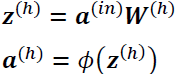
Here,  is our 1 × dimensional feature vector of a sample
 ![]() plus a bias unit.
plus a bias unit. ![]() is an × dimensional weight matrix where d is the number of units in the
is an × dimensional weight matrix where d is the number of units in the
hidden layer. After matrix-vector multiplication, we obtain the 1 × dimensional net input vector ![]() to calculate the activation
to calculate the activation ![]() (where
(where ![]() ∈
∈![]() ) .
) .
Furthermore, we can generalize this computation to all n examples in the training dataset: ![]()
Here, ![]() is now an × matrix, and the matrix-matrix multiplication will result in an × dimensional net input matrix
is now an × matrix, and the matrix-matrix multiplication will result in an × dimensional net input matrix ![]() . Finally, we apply the activation function (∙) to each value in the net input matrix to get the × activation matrix the next layer (here, the output layer):
. Finally, we apply the activation function (∙) to each value in the net input matrix to get the × activation matrix the next layer (here, the output layer):![]()
Similarly, we can write the activation of the output layer in vectorized form for multiple examples: ![]()
Here, we multiply the × matrix ![]() (t is the number of output units) by the × dimensional matrix
(t is the number of output units) by the × dimensional matrix ![]() to obtain the × dimensional matrix
to obtain the × dimensional matrix ![]() (the columns in this matrix represent the outputs for each sample).
(the columns in this matrix represent the outputs for each sample).
Lastly, we apply the sigmoid activation function to obtain the continuous valued output of our network: ![]()
Classifying handwritten digits
In the previous section, we covered a lot of the theory around NNs, which can be a little bit overwhelming if you are new to this topic. Before we continue with the discussion of the algorithm for learning the weights of the MLP model, backpropagation, let's take a short break from the theory and see an NN in action.
Additional resources on backpropagation
The NN theory can be quite complex; thus, it is recommended that you refer to two additional resources, which cover some of the concepts that we discuss in this chapter in more detail:
- • Chapter 6, Deep Feedforward Networks, Deep Learning, I. Goodfellow, Y. Bengio, and A. Courville, MIT Press, 2016 (Manuscripts freely accessible at http://www.deeplearningbook.org).
- • Pattern Recognition and Machine Learning, C. M. Bishop and others, Volume 1. Springer New York, 2006.
- • Lecture slides from the deep learning course at the University of Wisconsin–Madison:
- 1. https://sebastianraschka.com/pdf/lecture-notes/stat479ss19/L08_logistic_slides.pdf
- 2. https://sebastianraschka.com/pdf/lecture-notes/stat479ss19/L09_mlp_slides.pdf
In this section, we will implement and train our first multilayer NN to classify handwritten digits from the popular Mixed National Institute of Standards and Technology (MNIST) dataset that has been constructed by Yann LeCun and others and serves as a popular benchmark dataset for machine learning algorithms (Gradient-Based Learning Applied to Document Recognition, Y. LeCun, L. Bottou, Y.Bengio, and P. Haffner, Proceedings of the IEEE, 86(11): 2278-2324, November 1998).
Obtaining and preparing the MNIST dataset
The MNIST dataset is publicly available at http://yann.lecun.com/exdb/mnist/ and consists of the following four parts:
- • Training dataset images: train-images-idx3-ubyte.gz (9.9 MB, 47 MB unzipped, and 60,000 examples)
- • Training dataset labels: train-labels-idx1-ubyte.gz (29 KB, 60 KB unzipped, and 60,000 labels)
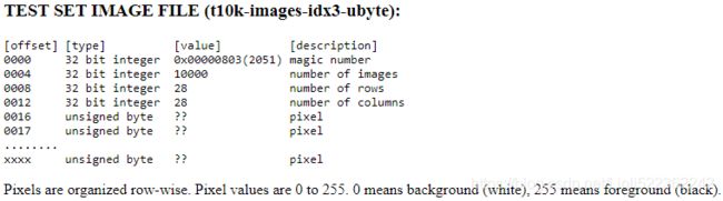
- • Test dataset images: t10k-images-idx3-ubyte.gz (1.6 MB, 7.8 MB unzipped, and 10,000 examples)
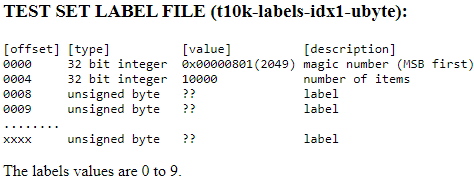
- • Test dataset labels: t10k-labels-idx1-ubyte.gz (5 KB, 10 KB unzipped, and 10,000 labels)

The MNIST dataset was constructed from two datasets of the US National Institute of Standards and Technology (NIST). The training dataset consists of handwritten digits from 250 different people, 50 percent high school students and 50 percent employees from the Census Bureau. Note that the test dataset contains handwritten digits from different people following the same split.
In this section, we will only be working with a subset of MNIST, thus, we only need to download the training set images and training set labels.
After downloading the files, simply run the next code cell to unzip the files.
import sys
import gzip
import shutil
import os

sys.version_info ![]()
os.chdir(r'C:\Users\LlQ\0Python Machine Learning\mnist')
os.getcwd() ![]()
if ( sys.version_info >(3,0) ):
    writemode='wb'
else:
    writemode='w'

zipped_mnist = [f for f in os.listdir() if f.endswith('ubyte.gz')]
for z in zipped_mnist:
    with gzip.GzipFile(z, mode='rb') as decompressed, open(z[:-3], writemode) as outfile:
outfile.write( decompressed.read() ) 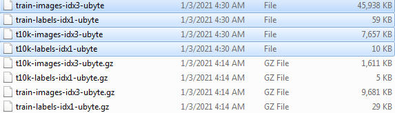
%ls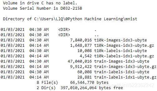
gzip *ubyte.gz -dAlternatively, you can use your favorite unzipping tool if you are working with a machine running Microsoft Windows.
1.1 struct.pack(fmt,v1,v2,.....)
将v1,v2等参数的值进行一层包装,包装的方法由fmt指定。被包装的参数必须严格符合fmt。最后返回一个包装后的字符串。
1.2 struct.unpack(fmt,string)
顾名思义,解包。比如pack打包,然后就可以用unpack解包了。返回一个由解包数据(string)得到的一个元组(tuple), 即使仅有一个数据也会被解包成元组。其中len(string) 必须等于 calcsize(fmt),这里面涉及到了一个calcsize函数。struct.calcsize(fmt):这个就是用来计算fmt格式所描述的结构的大小。
格式字符串(format string)由一个或多个格式字符(format characters)组成,对于这些格式字符的描述参照Python manual如下: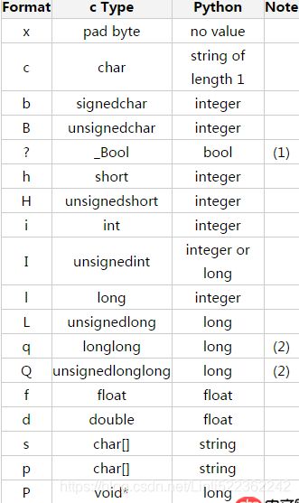
The images are stored in byte format, and we will read them into NumPy arrays that we will use to train and test our MLP implementation. In order to do that, we will define the following helper function:
import os
import struct
import numpy as np

def load_mnist( path, kind='train' ):
    """Load Mnist data from 'path'"""
    labels_path = os.path.join( path,
                                '%s-labels-idx1-ubyte' % kind)
    images_path = os.path.join( path,
                                '%s-images-idx3-ubyte' % kind)

    with open(labels_path, 'rb') as lbpath:
        magic, n = struct.unpack( '>II', # II: 2 unsigned integers and 1 unsigned integer = 2 bytes=16 bits
                                  lbpath.read(8) )#data start: 8
        # print(magic, n) # 2049(==0x00000801,0000 is a magic number; 08: data type is unsigned byte, 01: vector) 60000(vector) # OR 2049 10000
        labels = np.fromfile( lbpath,
                              dtype=np.uint8 )

    with open(images_path, 'rb') as imgpath:
        magic, num, rows, cols = struct.unpack( ">IIII", # 16 <== IIII
                                                imgpath.read(16) ) #data start: 16
        # print(magic, num, rows, cols) # 2051(0x00000803==,0000 is a magic number; 08: data type is unsigned byte, 03: 3D ) 60000 28 28 (3D) # OR 2051 10000 28 28
        images = np.fromfile( imgpath,
                              dtype=np.uint8).reshape( len(labels), 784 ) #784=28*28 #np.uint8,也就是0~255
        images = ( (images/255.)-.5 )*2
return images, labels 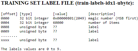

Using the two preceding lines of code, we first read in the magic number, which is a description of the file protocol, as well as the number of items (n) from the file buffer, before we load the following bytes into a NumPy array using the fromfile method. The fmt parameter value, '>II', that we passed as an argument to struct. unpack can be composed into the two following parts:
THE IDX(X=1, 2, 3, ...) FILE FORMAT
the IDX file format is a simple format for vectors and multidimensional matrices of various numerical types.
The basic format is
magic number
size in dimension 0
size in dimension 1
size in dimension 2
.....
size in dimension N
data
The magic number is an integer (MSB first). The first 2 bytes are always 0.
0000 32 bit integer 0x00000801(2049) magic number (MSB first)
0004 32 bit integer 60000 number of items
0008 unsigned byte ?? label
0000 32 bit integer 0x00000803(2051) magic number
0004 32 bit integer 60000 number of images
0008 32 bit integer 28 number of rows
0012 32 bit integer 28 number of columns
0016 unsigned byte ?? pixel
The third byte codes the type of the data:
0x08: unsigned byte
0x09: signed byte
0x0B: short (2 bytes)
0x0C: int (4 bytes)
0x0D: float (4 bytes)
0x0E: double (8 bytes)
The 4-th byte codes the number of dimensions of the vector/matrix: 1 for vectors( idx1), 2 for matrices, 3(e.g. 6000x28x28, idx3)
The sizes in each dimension are 4-byte integers (4*8=32, MSB first, high endian, like in most non-Intel processors).
The data is stored like in a C array, i.e. the index in the last dimension changes the fastest.
The load_mnist function returns two arrays, the first being an × dimensional NumPy array (images), where n is the number of examples and m is the number of features (here, pixels). The training dataset consists of 60,000 training digits and the test dataset contains 10,000 examples, respectively.
The images in the MNIST dataset consist of 28 × 28 pixels, and each pixel is represented by a grayscale intensity value. Here, we unroll the 28 × 28 pixels into one-dimensional row vectors, which represent the rows in our images array (784 per row or image). The second array (labels) returned by the load_mnist function contains the corresponding target variable, the class labels (integers 0-9) of the handwritten digits.
###############################
The way we read in the image might seem a little bit strange at first:
struct.unpack(fmt, string),该函数返回一个元组
        magic, n = struct.unpack( '>II',
                                  lbpath.read(8) )
        labels = np.fromfile( lbpath,
                              dtype=np.uint8 )
To understand how those two lines of code work, let's take a look at the dataset description from the MNIST website:
Using the two preceding lines of code, we first read in the magic number, which is a description of the file protocol, as well as the number of items (n) from the file buffer, before we load the following bytes into a NumPy array using the fromfile method. The fmt parameter value, '>II', that we passed as an argument to struct. unpack can be composed into the two following parts:
- • >: This is big-endian—it defines the order in which a sequence of bytes is stored; if you are unfamiliar with the terms big-endian and littleendian, you can find an excellent article about Endianness on Wikipedia: https://en.wikipedia.org/wiki/Endianness

- • I: This is an unsigned integer
格式符"i"表示转换为int,'ii'表示有两个int变量。import struct # defaultencoding("utf-8") a = 20 b = 400 # pack str = struct.pack("ii", a, b) print( 'length: ', len(str) ) # length: 8 print( str ) # 乱码: � print( repr(str) ) # '\x14\x00\x00\x00\x90\x01\x00\x00' # unpack str2 = struct.unpack("ii", str) print( 'length: ', len(str2) ) # length: 2 print( str2 ) # (20, 400) print( repr(str2) ) # (20, 400)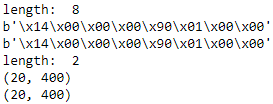
-
struct.calcsize
struct.calcsize用于计算格式字符串所对应的结果的长度,如:struct.calcsize('ii'),返回8。因为两个int类型所占用的长度是8个字节
import struct
print("len: ", struct.calcsize('i') )      # len:  4
print("len: ", struct.calcsize('ii') )      # len:  8
print("len: ", struct.calcsize('f') )       # len:  4
print("len: ", struct.calcsize('ff') )      # len:  8
print("len: ", struct.calcsize('s') )       # len:  1
print("len: ", struct.calcsize('ss') )      # len:  2
print("len: ", struct.calcsize('d') )       # len:  8
print("len: ", struct.calcsize('dd') )      # len:  1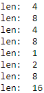
Finally, we also normalized the pixels values in MNIST to the range –1 to 1 (originally 0 to 255) via the following code line:
images = ( (images/255.)-.5 )*2The reason behind this is that gradient-based optimization is much more stable under these conditions as discussed in cp2_TrainingSimpleMachineLearningAlgorithmsForClassification_meshgrid_ravel_contourf_OvA_GradientDescent https://blog.csdn.net/Linli522362242/article/details/96429442. Note that we scaled the images on a pixel-by-pixel basis, which is different from the feature scaling approach that we took in previous chapters.
Previously, we derived scaling parameters from the training dataset and used these to scale each column in the training dataset and test dataset. However, when working with image pixels, centering them at zero(by '/255') and rescaling them to a [–1, 1](by -0.5 then *2 ) range is also common and usually works well in practice.
Batch normalization
A commonly used trick for improving convergence in gradient-based optimization through input scaling is batch normalization, which is an advanced topic that we will cover in
Chapter 17, Generative Adversarial Networks for Synthesizing New Data. Also, you can read more about batch normalization in the excellent research article Batch Normalization: Accelerating
Deep Network Training by Reducing Internal Covariate Shift by Sergey Ioffe and Christian Szegedy (2015, https://arxiv.org/abs/1502.03167).
###############################
By executing the following code, we will now load the 60,000 training instances as well as the 10,000 test examples from the local directory where we unzipped the MNIST dataset. (In the following code snippet, it is assumed that the downloaded MNIST files were unzipped to the same directory in which this code was executed.)
X_train, y_train = load_mnist(r'C:\Users\LlQ\0Python Machine Learning\mnist',
                              kind='train')
print('Rows: %d, columns: %d' % (X_train.shape[0], X_train.shape[1]) ) ![]()
X_test, y_test = load_mnist(r'C:\Users\LlQ\0Python Machine Learning\mnist',
                            kind='t10k')
print( 'Rows: %d, columns: %d' % (X_test.shape[0], X_test.shape[1]) )![]()
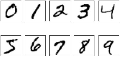
To get an idea of how those images in MNIST look, let's visualize examples of the digits 0-9 after reshaping the 784-pixel vectors from our feature matrix into the original 28 × 28 image that we can plot via Matplotlib's imshow function:
import matplotlib.pyplot as plt

fig, ax = plt.subplots( nrows=2, ncols=5, sharex=True, sharey=True)
ax = ax.flatten() # 2D==>1D
for i in range(10):
    img = X_train[y_train == i][0].reshape(28, 28) #[0] get the first row
    ax[i].imshow(img, cmap='Greys')

ax[0].set_xticks([])
ax[0].set_yticks([])
plt.tight_layout()

plt.show()
We should now see a plot of the 2 × 5 subfigures showing a representative image of each unique digit:
In addition, let's also plot multiple examples of the same digit to see how different the handwriting for each really is:
fig, ax = plt.subplots( nrows=5, ncols=5, sharex=True, sharey=True)
ax = ax.flatten()

for i in range(25):
    img = X_train[y_train==7][i].reshape(28,28)
    ax[i].imshow(img, cmap='Greys')

ax[0].set_xticks([])
ax[0].set_yticks([])
plt.tight_layout()

plt.show()
After executing the code, we should now see the first 25 variants of the digit 7:
After we've gone through all the previous steps, it is a good idea to save the scaled images in a format that we can load more quickly into a new Python session to avoid the overhead of reading in and processing the data again. When we are working with NumPy arrays, an efficient and convenient method to save multidimensional arrays to disk is NumPy's savez function. (The official documentation can be found here: https://docs.scipy.org/doc/numpy/reference/generated/numpy.savez.html.)
in cp9_Embedding aModel into a Web Application_pickle_sqlite3_Flask_wtforms_python any where_pickle_seria https://blog.csdn.net/Linli522362242/article/details/110740856, but optimized for storing NumPy arrays. The savez function creates zipped archives of our data, producing .npz files that contain files in the .npy format; if you want to learn more about this format, you can find a nice explanation, including a discussion about advantages and disadvantages, in the NumPy documentation: https://docs.scipy.org/doc/numpy/neps/npy-format.html. Furthermore, instead of using savez, we will use savez_compressed, which uses the same syntax as savez, but further compresses the output file down to substantially smaller file sizes (approximately 22 MB versus approximately 400 MB in this case). The following code snippet will save both the training and test datasets to the archive file mnist_scaled.npz:
import numpy as np

np.savez_compressed( 'mnist_scaled.npz',
                    X_train=X_train,
                    y_train=y_train,
                    X_test = X_test,
y_test = y_test )![]()
After we create the .npz files, we can load the preprocessed MNIST image arrays using NumPy's load function as follows:
mnist = np.load('mnist_scaled.npz')
mnist.files
The mnist variable now refers to an object that can access the four data arrays that we provided as keyword arguments to the savez_compressed function. These input arrays are now listed under the files attribute list of the mnist object:
![]()
For instance, to load the training data into our current Python session, we will access the X_train array as follows (similar to a Python dictionary):
X_train = mnist['X_train']Using a list comprehension, we can retrieve all four data arrays as follows
X_train, y_train, X_test, y_test = [mnist[f] for f in ['X_train', 'y_train', 'X_test', 'y_test'] ]

del mnist

X_train.shape![]()
Note that while the preceding np.savez_compressed and np.load examples are not essential for executing the code in this chapter, they serve as a demonstration of how to save and load NumPy arrays conveniently and efficiently.
Loading MNIST using scikit-learn
Using scikit-learn's new fetch_openml function, it is now also possible to load the MNIST dataset more conveniently. For example, you can use the following code to create a 50,000-example training dataset and and a 10,000-example test dataset by fetching the dataset from https://www.openml.org/d/554:
from sklearn.datasets import fetch_openml
from sklearn.model_selection import train_test_split

X, y = fetch_openml( 'mnist_784', version=1, return_X_y=True )
y = y.astype(int)
X = ( (X/255.)-0.5)*2
X_train, X_test, y_train, y_test = train_test_split( X,y, test_size=10000, random_state=123, stratify=y)

X_train.shape![]()
Please note that the distribution of MNIST records into training and test datasets will be different from the manual approach outlined in this section. Thus, you will observe slightly different
results in the following sections if you load the dataset using the fetch_openml and train_test_split functions.
Implementing a multilayer perceptron
In this subsection, we will now implement an MLP from scratch to classify the images in the MNIST dataset. To keep things simple, we will implement an MLP with only one hidden layer. Since the approach may seem a little bit complicated at first, you are encouraged to download the sample code for this chapter from the Packt Publishing website or from GitHub (https://github.com/rasbt/
python-machine-learning-book-3rd-edition) so that you can view this MLP implementation annotated with comments and syntax highlighting for better readability.
If you are not running the code from the accompanying Jupyter Notebook file or don't have access to the Internet, copy the NeuralNetMLP code from this chapter into a Python script file in your current working directory (for example, neuralnet.py), which you can then import into your current Python session via the following command:
from neuralnet import NeuralNetMLPThe code will contain parts that we have not talked about yet, such as the backpropagation algorithm, but most of the code should look familiar to you based on the Adaline implementation in cp2_TrainingSimpleMachineLearningAlgorithmsForClassification_meshgrid_ravel_contourf_OvA_GradientDescent https://blog.csdn.net/Linli522362242/article/details/96429442, and the discussion of forward propagation in earlier sections.
Do not worry if not all of the code makes immediate sense to you; we will follow up on certain parts later in this chapter. However, going over the code at this stage can make it easier to follow the theory later.
The following is the implementation of an MLP(forward propagation and back propagation):
https://blog.csdn.net/Linli522362242/article/details/104070847 04_TrainingModels_02_regularization_L2_cost_Ridge_Lasso_Elastic Net_Early Stopping

 and
and 
 ==>sigmoid_derivative_h = a_h * (1.- a_h) <== a_h = 1. / ( 1.+ np.exp( z ) ) <==z_h = np.dot( X, self.w_h ) + self.b_h
Next:


############################################
Equation 4-18. Logistic cost function partial derivatives https://blog.csdn.net/Linli522362242/article/details/104070847
In neuralnet.py, we not use MSE as cost function we use 1/2* SE(sum square of error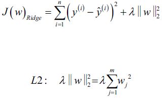 ), so Logistic cost function partial derivatives :
 ==> Derivation of weights = 1/2 * 2* Lambda_2 * weight =Lambda_2 * weight , remove 2 since cost function is 1/2* SE(sum square of error)
use RSS(Residuals of Sum Squares) instead of MSE, the correct formula:
# -*- coding: utf-8 -*-
"""
Created on Sun Jan  3 22:28:03 2021

@author: LlQ
"""

import numpy as np
import sys

class NeuralNetMLP( object ):
    """Feedforward nural network /Multi-layer perceptron classifier

    Parameters
    ------------
    n_hidden : int(default: 30)
               Number of hidden units.
    l2 : float (default: 0.)
         Lambda value for L2-regularization.
         No regularization if l2=0. (default)
    epochs : int (default: 100)
             Number of passes over the training set.
    eta : float (default: 0.001)
          Learning rate.
    shuffle : bool (default: True)
              Shuffles training data every epoch if True to prevent circles.
    minibatch_size : int(default: 1)
        Number of training examples per minibatch.
    seed : int (default: None)
           Random seed for initializing weights and shuffling.

    Attributes
    -----------
    eval_ : dict
            Dictionary collecting the cost, training accuracy,
            and validation accuracy for each epoch during training.
    """
    def __init__( self, n_hidden=30,
                  l2=0., epochs=100, eta=0.001,
                  shuffle=True, minibatch_size=1, seed=None ):
        self.random = np.random.RandomState( seed )
        self.n_hidden = n_hidden
        self.l2 = l2
        self.epochs = epochs
        self.eta = eta
        self.shuffle = shuffle
        self.minibatch_size = minibatch_size

    def _onehot( self, y, n_classes ):
        """Encode labels into one-hot representation

        Parameters
        -----------
        y : array, shape=[n_examples]
            Target values.
        n_classes : int
                    Number of classes

        Returns
        -----------
        onehot : array, shape = (n_examples, n_labels)
        """
        onehot = np.zeros( ( n_classes, y.shape[0] ) )
        for idx, val in enumerate( y.astype(int) ):
            onehot[val, idx] = 1.
        return onehot.T

    def _sigmoid( self, z ):
        """Compute logistic function (sigmoid) phi(Z) = 1/(1+e^-Z) Z=W^T * X"""
        return 1. / ( 1.+ np.exp( -np.clip(z, -250, 250) ) )

    def _forward( self, X ):
        """Compute forward propagation step"""

        # step 1: net input of hidden layer(n_hidden is the number of neurons)
        #         [n_examples, n_features] dot [n_features, n_hidden]
        #       ==> [n_examples, n_hidden]
        z_h = np.dot( X, self.w_h ) + self.b_h

        # step 2: activation of hidden layer
        a_h = self._sigmoid( z_h ) # S-shape

        # step 3: net input of output layer
        #         [n_examples, n_hidden] dot [n_hidden, n_classlabels]
        #       ==> [n_examples, n_classlabels]
        z_out = np.dot(a_h, self.w_out) + self.b_out

        # step 4: activation output layer
        a_out = self._sigmoid(z_out)

        return z_h, a_h, z_out, a_out

    def _compute_cost( self, y_enc, output ):
        """Compute cost function

        Parameters
        -----------
        y_enc : array, shape = (n_examples, n_labels)
                one-hot encoded class labels.
        output : array, shape = [n_examples, n_output_units]
                 Activation of the output layer (forward propagation)

        Returns
        -----------
        cost : float
               Regularized cost
        """
        L2_term = ( self.l2 * ( np.sum( self.w_h ** 2. ) ) )
        term1 = -y_enc*( np.log(output) )
        term2 = (1. -y_enc) * np.log(1.-output)
        cost = np.sum( term1 - term2 ) + L2_term

        # If you are applying this cost function to other datasets where
        # activation values maybe become more extreme (closer to zero or 1)
        # you may enconter "ZeroDivisionError"s due to numerical instabilities
        # in Python & NumPy for the current implementation.
        # I.e., the code tries to evaluate log(0), which is undefined.
        # To address this issue, you could add a small constant to the
        # activation values that are passed to the log function.
        #
        # For example:
        #
        # term1 = -y_enc * ( np.log(output - 1e-5) )
        # term2 = (1. - y_enc) * np.log(1.-output + 1e-5)

        return cost

    def predict( self, X ):
        """Predict class labels

        Parameters
        -----------
        X : array, shape = [n_examples, n_features]
            Input layer with original features.

        Returns:
        y_pred : array, shape=[n_examples]
                 Predicted class labels.
        """
        z_h, a_h, z_out, a_out = self._forward(X)
        # z_out.shape ==> [n_examples, n_classlabels]
        y_pred = np.argmax( z_out, axis=1 )
        return y_pred

    def fit( self, X_train, y_train, X_valid, y_valid ):
        """Learn weights from traning data

        Parameters
        -----------
        X_train : array, shape = [n_examples, n_features]
                  Input layer with original features.
        y_train : array, shape = [n_examples]
                  Target class labels.
        X_valid : array, shape = [n_examples, n_features]
                  Sample features for validation during training
        y_valid : array, shape = [n_examples]
                  Sample labels for validation during training

        Returns:
        -----------
        self
        """
        n_output = np.unique( y_train ).shape[0] # number of class labels
        n_features = X_train.shape[1]

        ########################
        # Weight initialization
        ########################

        # weights for input -> hidden
        self.b_h = np.zeros( self.n_hidden )
        self.w_h = self.random.normal( loc=0.0, scale=0.1, # μ=0, σ=1 # scale越大越矮胖,scale越小,越瘦高
                                       size=(n_features, self.n_hidden) )
        # weights for hidden -> output
        self.b_out = np.zeros(n_output)
        self.w_out = self.random.normal( loc=0.0, scale=0.1,
                                         size=(self.n_hidden, n_output) )


        epoch_strlen = len( "%s" % self.epochs ) # for progress formatting

        self.eval_ = { 'cost':[], 'train_acc':[], 'valid_acc':[] }

        y_train_enc = self._onehot( y_train, n_output)


        ########################
        # Iteration process --- mini-batch learning
        ########################
        # iterate over training epochs
        for i in range( self.epochs ):
            # iterate over minibatches
            indices = np.arange(X_train.shape[0])

            if self.shuffle:
                self.random.shuffle( indices )

            for start_idx in range(0,
                                   indices.shape[0] - self.minibatch_size + 1,
                                   self.minibatch_size):
                batch_idx = indices[start_idx: start_idx + self.minibatch_size]

                # forward propagation
                z_h, a_h, z_out, a_out = self._forward(X_train[batch_idx])

                ##################
                # Backpropagation
                ##################

                # self.w_out.shape : (self.n_hidden, n_output)
                # [n_examples, n_classlabels] # n_output==n_classlabels
                delta_out = a_out - y_train_enc[batch_idx]

                # [n_examples, n_hidden]
                # sigmoid: a_h = 1. / ( 1.+ np.exp( z ) )
                sigmoid_derivative_h = a_h * (1.- a_h) #<== derivative of a_h

                # [n_examples, n_classlabels] dot [n_classlabels, n_hidden]
                # ==> [n_examples, n_hidden]
                # Logistic cost function partial derivatives
                # https://blog.csdn.net/Linli522362242/article/details/104070847

                # z_h = np.dot( X, self.w_h ) + self.b_h       ###############
                # a_h = self.sigmoid( z_h )                    ###############
                # z_out = np.dot(a_h, self.w_out) + self.b_out
                ########### wi = w + delta_wi and delta_wi = 1*(y-y_pred)*X
                delta_h = ( np.dot(delta_out,
                                   self.w_out.T)
                            * sigmoid_derivative_h ) #########################

                # [n_features, n_examples] dot [n_examples, n_hidden]
                # ==> [n_features, n_hidden]
                grad_w_h = np.dot(X_train[batch_idx].T, delta_h)
                grad_b_h = np.sum(delta_h, axis=0)

                # [n_hidden, n_examples] dot [n_examples, n_classlabels]
                # ==> [n_hidden, n_classlabels]
                grad_w_out = np.dot(a_h.T, delta_out)            # delta_wi = 1*(y-y_pred)*X
                grad_b_out = np.sum(delta_out, axis=0)           # delta_w0 = 1*(y-y_pred)*1

                # Regularization and weight updates
                delta_w_h = ( grad_w_h + self.l2 * self.w_h )
                delta_b_h = grad_b_h # bias is not regularized

                self.w_h -= self.eta * delta_w_h
                self.b_h -= self.eta * delta_b_h

                delta_w_out = ( grad_w_out + self.l2*self.w_out )
                delta_b_out = grad_b_out # bias is not regularized

                self.w_out -= self.eta * delta_w_out
                self.b_out -= self.eta * delta_b_out

            # end inner for loop #in mini batch learning

            #############
            # Evaluation
            #############

            # Evaluation after each epoch during training
            z_h, a_h, z_out, a_out = self._forward(X_train)
            cost = self._compute_cost( y_enc = y_train_enc,
                                       output = a_out )
            y_train_pred = self.predict(X_train)
            y_valid_pred = self.predict(X_valid)

            train_acc = ( ( np.sum(y_train == y_train_pred)
                          ).astype(np.float)/X_train.shape[0] )

            valid_acc = ( ( np.sum(y_valid == y_valid_pred)
                          ).astype(np.float)/X_valid.shape[0] )

            sys.stderr.write('\r%0*d/%d | Cost: %.2f '
                             '| Train/Valid Acc.: %.2f%%/%.2f%% ' %
                             (epoch_strlen, i+1, self.epochs, cost,
                              train_acc*100, valid_acc*100))
            sys.stderr.flush()

            self.eval_['cost'].append(cost)
            self.eval_['train_acc'].append(train_acc)
            self.eval_['valid_acc'].append(valid_acc)
        return self
After executing this code, we next initialize a new 784-100-10 MLP—an NN with 784 input units (n_features), 100 hidden units (n_hidden), and 10 output units (n_output):
nn = NeuralNetMLP(n_hidden=100,
                  l2=0.01,
                  epochs=n_epochs,
                  eta=0.0005,
                  minibatch_size=100,
                  shuffle=True,
                  seed=1)
If you read through the NeuralNetMLP code, you've probably already guessed what these parameters are for. Here, you find a short summary of them:
- • l2: This is the parameter for L2 regularization to decrease the degree of overfitting.
- • epochs: This is the number of passes over the training dataset.
- • eta: This is the learning rate .
- • shuffle: This is for shuffling the training set prior to every epoch to prevent the algorithm getting stuck in circles.
- • seed: This is a random seed for shuffling and weight initialization.
- minibatch_size: This is the number of training examples in each minibatch when splitting the training data in each epoch for SGD. The gradient is computed for each mini-batch separately instead of the entire training data for faster learning.
Next, we train the MLP using 55,000 examples from the already shuffled MNIST training dataset and use the remaining 5,000 examples for validation during training. Note that training the NN may take up to five minutes on standard desktop computer hardware.
As you may have noticed from the preceding code, we implemented the fit method so that it takes four input arguments: training images, training labels, validation images, and validation labels. In NN training, it is really useful to compare training and validation accuracy, which helps us judge whether the network model performs well, given the architecture and hyperparameters. For example, if we observe a low training and validation accuracy, there is likely an issue with the training dataset, or the hyperparameters settings are not ideal. A relatively large gap between the training and the validation accuracy indicated that the model is likely overfitting the training dataset so that we want to reduce the number of parameters in the model or increase the regularization strength. If both the training and validation accuracies are high, the model is likely to generalize well to new data, for example, the test dataset, which we use for the final model evaluation.
In general, training (deep) NNs is relatively expensive compared with the other models we've discussed so far. Thus, we want to stop it early in certain circumstances and start over with different hyperparameter settings. On the other hand, if we find that it increasingly tends to overfit the training data (noticeable by an increasing gap between training and validation dataset performance), we may want to stop the training early as well.
Now, to start the training, we execute the following code:
nn.fit(X_train=X_train[:55000],
       y_train=y_train[:55000],
       X_valid=X_train[55000:],
y_valid=y_train[55000:])![]()
In our NeuralNetMLP implementation, we also defined an eval_ attribute that collects the cost, training, and validation accuracy for each epoch so that we can visualize the results using Matplotlib:
import matplotlib.pyplot as plt

plt.plot( range(nn.epochs), nn.eval_['cost'])
plt.ylabel('Cost')
plt.xlabel('Epochs')

plt.show()
The preceding code plots the cost over the 200 epochs, as shown in the following graph:
As we can see, the cost decreased substantially during the first 100 epochs and seems to slowly converge in the last 100 epochs. However, the small slope between epoch 175 and epoch 200 indicates that the cost would further decrease with a training over additional epochs.
Next, let's take a look at the training and validation accuracy:
plt.plot( range(nn.epochs), nn.eval_['train_acc'],
          label='Training', c='b')
plt.plot( range(nn.epochs), nn.eval_['valid_acc'],
          label='Validation', c='g')
plt.ylabel('Accuracy')
plt.xlabel('Epochs')
plt.legend( loc='lower right' )

plt.show()
The preceding code examples plot those accuracy values over the 200 training epochs, as shown in the following figure:
The plot reveals that the gap between training and validation accuracy increases as we train for more epochs.
Note that this example was chosen deliberately有意 to illustrate the effect of overfitting and demonstrate why it is useful to compare the validation and training accuracy values during training. One way to decrease the effect of overfitting is to increase the regularization strength—for example, by setting l2=0.1. Another useful technique to tackle overfitting in NNs is dropout, which will be covered in cp15_Classifying Images with Deep Convolutional NN_Loss_Cross Entropy_ax.text_mnist_ CelebA_Colab_ck https://blog.csdn.net/Linli522362242/article/details/108414534.
Finally, let's evaluate the generalization performance of the model by calculating the prediction accuracy on the test dataset:
y_test_pred = nn.predict(X_test)
acc = ( np.sum(y_test == y_test_pred).astype(np.float)/X_test.shape[0] )
print('Test accuracy: %.2f%%' % (acc*100) ) # %% for printing %![]()
Despite the slight overfitting on the training data, our relatively simple one-hidden-layer NN achieved a relatively good performance on the test dataset, similar to the validation dataset accuracy (97.38 percent).
To further fine-tune the model, we could change the number of hidden units, values of the regularization parameters, and the learning rate, or use various other tricks that have been developed over the years but are beyond the scope of this book. In Chapter 15, Classifying Images with Deep Convolutional Neural Networks, you will learn about a different NN architecture that is known for its good performance on image datasets. Also, the chapter will introduce additional performance-enhancing tricks such as adaptive learning rates, more sophisticated SGD-based optimization algorithms, batch normalization, and dropout.
Other common tricks that are beyond the scope of the following chapters include:
- • Adding skip-connections, which are the main contribution of residual NNs (Deep residual learning for image recognition. K. He, X. Zhang, S. Ren, J. Sun (2016). In Proceedings of the IEEE Conference on Computer Vision and Pattern Recognition, pp. 770-778)
- • Using learning rate schedulers that change the learning rate during training (Cyclical learning rates for training neural networks. L.N. Smith (2017). In 2017 IEEE Winter Conference on Applications of Computer Vision (WACV), pp. 464-472)
- • Attaching loss functions to earlier layers in the networks as it's being done in the popular Inception v3 architecture (Rethinking the Inception architecture for computer vision. C. Szegedy, V. Vanhoucke, S. Ioffe, J. Shlens, Z. Wojna (2016). In Proceedings of the IEEE Conference on Computer Vision and Pattern Recognition, pp. 2818-2826)
Lastly, let's take a look at some of the images that our MLP struggles with:
miscl_img = X_test[ y_test != y_test_pred ][:25]
correct_label = y_test[ y_test != y_test_pred ][:25]
miscl_label = y_test_pred[y_test!=y_test_pred][:25]

fig, ax=plt.subplots(nrows=5, ncols=5, sharex=True, sharey=True)
ax = ax.flatten()
for i in range(25):
    img = miscl_img[i].reshape(28,28)
    ax[i].imshow(img, cmap='Greys', interpolation='nearest')
    ax[i].set_title( '%d) t: %d p: %d' % (i+1, correct_label[i], miscl_label[i]) )

ax[0].set_xticks([])
ax[0].set_yticks([])
plt.tight_layout()
plt.show()
We should now see a 5 × 5 subplot matrix where the first number in the subtitles indicates the plot index, the second number represents the true class label (t), and the third number stands for the predicted class label (p):
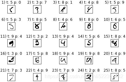
As we can see in the preceding figure, some of those images are even challenging for us humans to classify correctly. For example, the 9 in subplot 13 really looks like a carelessly drawn 4.
Training an artificial neural network
Now that we have seen an NN in action and have gained a basic understanding of how it works by looking over the code, let's dig a little bit deeper into some of the concepts, such as the logistic cost function and the backpropagation algorithm that we implemented to learn the weights.
Computing the logistic cost function
The logistic cost function that we implemented as the _compute_cost method is actually pretty simple to follow since it is the same cost function that we described in the logistic regression section in cp3 A Tour of ML Classifiers_stratify_bincount_likelihood_logistic regression_odds ratio_decay_L2 https://blog.csdn.net/Linli522362242/article/details/96480059:
Here, ![]() is the sigmoid activation of the ith sample in the dataset, which we compute in the forward propagation step:
is the sigmoid activation of the ith sample in the dataset, which we compute in the forward propagation step:![]()
Again, note that in this context, the superscript [i] is an index for training examples, not layers.
Now, let's add a regularization term, which allows us to reduce the degree of overfitting. As you recall from earlier chapters, the L2 regularization term is defined as follows (remember that we don't regularize the bias units):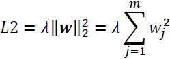
By adding the L2 regularization term to our logistic cost function, we obtain the following equation:
Previously, we implemented an MLP for multiclass classification that returns an output vector of t elements that we need to compare to the × 1 dimensional target vector in the one-hot encoding representation. If we predict the class label of an input image with class label 2, using this MLP, the activation of the third layer and the target may look like this:
Thus, we need to generalize the logistic cost function to all t activation units in our network. The cost function (without the regularization term) becomes the following: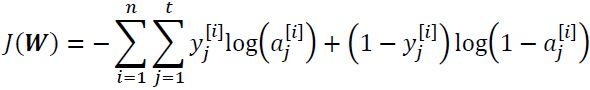
Here, again, the superscript [i] is the index of a particular sample in our training dataset.
The following generalized regularization term may look a little bit complicated at first, but here we are just calculating the sum of all weights of an l layer (without the bias term) that we added to the first column:
Here, ![]() refers to the number of units in a given layer l, and the following expression represents the penalty term:
refers to the number of units in a given layer l, and the following expression represents the penalty term: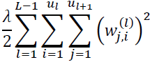
Remember that our goal is to minimize the cost function J(W); thus, we need to calculate the partial derivative of the parameters W with respect to each weight for every layer in the network: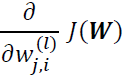
In the next section, we will talk about the backpropagation algorithm, which allows us to calculate those partial derivatives to minimize the cost function.
Note that W consists of multiple matrices. In an MLP with one hidden layer, we have the weight matrix, ![]() , which connects the input to the hidden layer, and
, which connects the input to the hidden layer, and ![]() , which connects the hidden layer to the output layer. A visualization of the threedimensional tensor W is provided in the following figure:
, which connects the hidden layer to the output layer. A visualization of the threedimensional tensor W is provided in the following figure: # [n_examples, n_features] dot [n_features, n_hidden] ==> [n_examples, n_hidden]https://blog.csdn.net/Linli522362242/article/details/106433059
In this simplified figure, it may seem that both ![]() and
and ![]() have the same number of rows and columns, which is typically not the case unless we initialize an MLP with the same number of hidden units, output units, and input features.
have the same number of rows and columns, which is typically not the case unless we initialize an MLP with the same number of hidden units, output units, and input features.
If this sounds confusing, stay tuned for the next section, where we will discuss the dimensionality of ![]() and
and ![]() in more detail in the context of the backpropagation algorithm. Also, you are encouraged to read through the code of the NeuralNetMLP again, which is annotated with helpful comments about the dimensionality of the different matrices and vector transformations. You can obtain the annotated code either from Packt or the book's GitHub repository at https://github.com/rasbt/python-machine-learning-book-3rd-edition.
in more detail in the context of the backpropagation algorithm. Also, you are encouraged to read through the code of the NeuralNetMLP again, which is annotated with helpful comments about the dimensionality of the different matrices and vector transformations. You can obtain the annotated code either from Packt or the book's GitHub repository at https://github.com/rasbt/python-machine-learning-book-3rd-edition.
Developing your understanding of backpropagation
Although backpropagation was rediscovered and popularized more than 30 years ago (Learning representations by back-propagating errors, D. E. Rumelhart, G. E. Hinton, and R. J. Williams, Nature, 323: 6088, pages 533–536, 1986), it still remains one of the most widely used algorithms to train artificial NNs very efficiently. If you are interested in additional references regarding the history of backpropagation, Juergen Schmidhuber wrote a nice survey article, Who Invented Backpropagation?, which you can find online at http://people.idsia.ch/~juergen/who-inventedbackpropagation.html.
This section will provide both a short, clear summary and the bigger picture of how this fascinating algorithm works before we dive into more mathematical details. In essence, we can think of backpropagation as a very computationally efficient approach to compute the partial derivatives of a complex cost function in multilayer NNs. Here, our goal is to use those derivatives to learn the weight coefficients for parameterizing such a multilayer artificial NN. The challenge in the parameterization of NNs. is that we are typically dealing with a very large number of weight coefficients in a high-dimensional feature space. In contrast to cost functions of single-layer NNs such as Adaline or logistic regression, which we have seen in previous chapters, the error surface of an NN cost function is not convex or smooth with respect to the parameters. There are many bumps in this high-dimensional cost surface (local minima) that we have to overcome in order to find the global minimum of the cost function.
You may recall the concept of the chain rule from your introductory calculus classes. The chain rule is an approach to compute the derivative of a complex, nested function, such as f ( g(x)), as follows:
Similarly, we can use the chain rule for an arbitrarily long function composition. For example, let's assume that we have five different functions, f(x), g(x), h(x), u(x), and v(x), and let F be the function composition: F(x) = f(g(h(u(v(x))))). Applying the chain rule, we can compute the derivative of this function as follows:
In the context of computer algebra, a set of techniques has been developed to solve such problems very efficiently, which is also known as automatic differentiation. If you are interested in learning more about automatic differentiation(09_Up and Running with TensorFlow_2_Autodiff_momentum optimizer_Mini-batchGradientDescent_SavingMode https://blog.csdn.net/Linli522362242/article/details/106290394) in machine learning applications, read A. G. Baydin and B. A. Pearlmutter's article Automatic Differentiation of Algorithms for Machine Learning, arXiv preprint arXiv:1404.7456, 2014, which is freely available on arXiv at http://arxiv.org/pdf/1404.7456.pdf.
##########################################################################https://blog.csdn.net/Linli522362242/article/details/106290394
Forward-Mode Autodiff前向自动积分
Forward-mode autodiff is neither numerical differentiation nor symbolic differentiation, but in some ways it is their love child. It relies on dual numbers对偶数, which are (weird but fascinating) numbers of the form a + bϵ where a and b are real numbers and ϵ is an infinitesimal [ˌɪnfɪnɪˈtesɪml]无限小地 number such that ![]() = 0 (but ϵ ≠ 0). You can think of the dual number 42 + 24ϵ as something akin相似的 to 42.0000⋯000024 with an infinite number of 0s (but of course this is simplified just to give you some idea of what dual numbers are). A dual number is represented in memory as a pair of floats. For example, 42 + 24ϵ is represented by the pair (42.0, 24.0).
= 0 (but ϵ ≠ 0). You can think of the dual number 42 + 24ϵ as something akin相似的 to 42.0000⋯000024 with an infinite number of 0s (but of course this is simplified just to give you some idea of what dual numbers are). A dual number is represented in memory as a pair of floats. For example, 42 + 24ϵ is represented by the pair (42.0, 24.0).
Dual numbers can be added, multiplied, and so on, as shown in Equation D-3.
Equation D-3. A few operations with dual numbers
 (since
 ![]() = 0 )
= 0 )
Most importantly, it can be shown that h(a + bϵ) = h(a) + b × h′(a)ϵ, so computing h(a + ϵ) gives you both h(a) and the derivative h′(a) in just one shot. Figure D-2 shows how forward-mode autodiff computes the partial derivative of f(x,y)= with regards to x at x = 3 and y = 4. All we need to do is compute f(3 + ϵ, 4); this will output a dual number whose first component is equal to f(3, 4) and whose second component is equal to
 ![]() .
.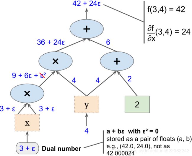 Figure D-2. Forward-mode autodiff
To compute ![]() =10 we would have to go through the graph again, but this time with x = 3 and y = 4 + ϵ.
=10 we would have to go through the graph again, but this time with x = 3 and y = 4 + ϵ.
So forward-mode autodiff is much more accurate than numerical differentiation, but it suffers from the same major flaw缺点: if there were 1,000 parameters, it would require 1,000 passes through the graph to compute all the partial derivatives. This is where reverse-mode autodiff shines: it can compute all of them in just two passes through
the graph.
Reverse-Mode Autodiff
Reverse-mode autodiff is the solution implemented by TensorFlow.
- It first goes through the graph in the forward direction (i.e., from the inputs to the output) to compute the value of each node.
- Then it does a second pass, this time in the reverse direction (i.e., from the output to the inputs) to compute all the partial derivatives.
 Figure D-3. Reverse-mode autodiff
Figure D-3 represents the second pass. During the first pass, all the node values were computed, starting from x = 3 and y = 4. You can see those values at the bottom right of each node (e.g., ![]() : x × x =3 × 3= 9,
: x × x =3 × 3= 9,![]() × y = 9 × 4 = 36, y + 2 = 4 + 2 = 6, 36 + 6 = 42 ). The nodes are labeled n1 to n7 for clarity. The output node is
× y = 9 × 4 = 36, y + 2 = 4 + 2 = 6, 36 + 6 = 42 ). The nodes are labeled n1 to n7 for clarity. The output node is ![]() : f(3,4) =
: f(3,4) =  = 42.
= 42.
The idea is to gradually go down the graph, computing the partial derivative of f(x,y) with regards to each consecutive node, until we reach the variable nodes. For this, reverse-mode autodiff relies heavily on the chain rule, shown in Equation D-4.
Equation D-4. Chain rule 
Since is the output node, f = so trivially ![]() = 1.
= 1.
Let's continue down the graph to ![]() : how much does f vary when
: how much does f vary when ![]() varies? The answer is
varies? The answer is  . We already know that
  = 1, so all we need is
 ![]() . Since simply performs the sum
. Since simply performs the sum  =, we find that
  , so
, so  .
.
Now we can proceed to node ![]() : how much does f vary when
: how much does f vary when ![]() varies? The answer is
varies? The answer is  . Since
 ![]() , we find that
, we find that  , so
, so ![]() .
.
The process continues until we reach the bottom of the graph. At that point we will have calculated all the partial derivatives of f(x,y) at the point x = 3 and y = 4. In this example, we find ∂f/∂x = ![]() and ∂f/∂y =
and ∂f/∂y =  . Sounds about right!
Reverse-mode autodiff is a very powerful and accurate technique, especially when there are many inputs and few outputs, since it requires only one forward pass plus one reverse pass per output to compute all the partial derivatives for all outputs with regards to all the inputs. Most importantly, it can deal with functions defined by arbitrary code. It can also handle functions that are not entirely differentiable, as long as you ask it to compute the partial derivatives at points that are differentiable.
##########################################################################
Automatic differentiation comes with two modes, the forward and reverse modes; backpropagation is simply a special case of reverse-mode automatic differentiation. The key point is that applying the chain rule in the forward mode could be quite expensive since we would have to multiply large matrices for each layer (Jacobians) that we would eventually multiply by a vector to obtain the output.
The trick of reverse mode is that we start from right to left: we multiply a matrix by a vector, which yields another vector that is multiplied by the next matrix and so on. Matrix-vector multiplication is computationally much cheaper than matrix-matrix multiplication, which is why backpropagation is one of the most popular algorithms used in NN training.
A basic calculus refresher
To fully understand backpropagation, we need to borrow certain concepts from differential calculus, which is outside the scope of this book. However, you can refer to a review chapter of the most fundamental concepts, which you might find useful in this context. It discusses function derivatives, partial derivatives, gradients, and the Jacobian. This text is freely accessible at https://sebastianraschka.com/pdf/books/dlb/appendix_d_calculus.pdf. If you are unfamiliar with calculus or need a brief refresher, consider reading this text as an additional supporting resource before reading the next section.
Training neural networks via backpropagation
In this section, we will go through the math of backpropagation to understand how you can learn the weights in an NN very efficiently. Depending on how comfortable you are with mathematical representations, the following equations may seem relatively complicated at first.
In a previous section, we saw how to calculate the cost as the difference between the activation of the last layer and the target class label. Now, we will see how the backpropagation algorithm works to update the weights in our MLP model from a mathematical perspective, which we implemented after the # Backpropagation code comment inside the fit method. As we recall from the beginning of this chapter, we first need to apply forward propagation in order to obtain the activation of the output layer, which we formulated as follows: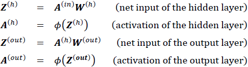
Concisely, we just forward-propagate the input features through the connection in the network, as shown in the following illustration: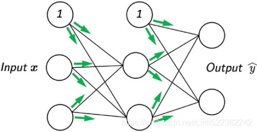
In backpropagation, we propagate the error from right to left. We start by calculating the error vector of the output layer:![]()
Here, y is the vector of the true class labels (the corresponding variable in the NeuralNetMLP code is delta_out).
Next, we calculate the error term of the hidden layer:
Here,  is simply the derivative of the sigmoid activation function, which we computed as sigmoid_derivative_h = a_h * (1. - a_h) in the fit method of the NeuralNetMLP:
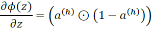
Note that the ⊙ symbol means element-wise multiplication in this context.
Activation function derivative
Although it is not important to follow the next equations, you may be curious how the derivative of the activation function was obtained; it is summarized step by step here: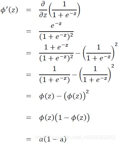 OR
OR
 and
and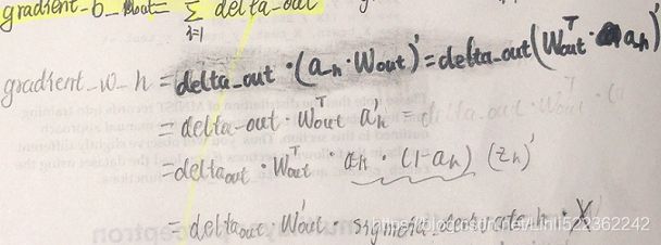
Next, we compute the ![]() layer error matrix (delta_h) as follows:
layer error matrix (delta_h) as follows:![]()
To better understand how we computed this ![]() term, let's walk through it in more detail. In the preceding equation, we used the transpose
term, let's walk through it in more detail. In the preceding equation, we used the transpose ![]() of the
of the
ℎ × -dimensional matrix ![]() . Here, t is the number of output class labels and h is the number of hidden units. The matrix multiplication between the × - dimensional
. Here, t is the number of output class labels and h is the number of hidden units. The matrix multiplication between the × - dimensional ![]() matrix and the × ℎ- dimensional matrix
matrix and the × ℎ- dimensional matrix![]() results in an × ℎ -dimensional matrix that we multiplied element-wise by the sigmoid derivative of the same dimension to obtain the × ℎ- dimensional matrix
results in an × ℎ -dimensional matrix that we multiplied element-wise by the sigmoid derivative of the same dimension to obtain the × ℎ- dimensional matrix ![]() .
.
Eventually, after obtaining the terms, we can now write the derivation of the cost function as follows:
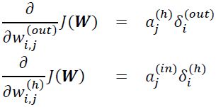
Next, we need to accumulate the partial derivative of every node in each layer and the error of the node in the next layer. However, remember that we need to compute![]() for every sample in the training dataset. Thus, it is easier to implement it as a vectorized version like in our NeuralNetMLP code implementation:
for every sample in the training dataset. Thus, it is easier to implement it as a vectorized version like in our NeuralNetMLP code implementation: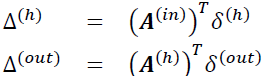
And after we have accumulated the partial derivatives, we can add the following regularization term:![]()
(Please note that the bias units are usually not regularized.)
The two previous mathematical equations correspond to the code variables delta_w_h, delta_b_h, delta_w_out, and delta_b_out in NeuralNetMLP.
Lastly, after we have computed the gradients, we can update the weights by taking an opposite step toward the gradient for each layer l:![]()
This is implemented as follows:
                # Regularization and weight updates
                delta_w_h = ( grad_w_h + self.l2 * self.w_h )
                delta_b_h = grad_b_h # bias is not regularized

                self.w_h -= self.eta * delta_w_h
                self.b_h -= self.eta * delta_b_h

                delta_w_out = ( grad_w_out + self.l2*self.w_out )
                delta_b_out = grad_b_out # bias is not regularized

                self.w_out -= self.eta * delta_w_out
                self.b_out -= self.eta * delta_b_out
To bring everything together, let's summarize backpropagation in the following figure: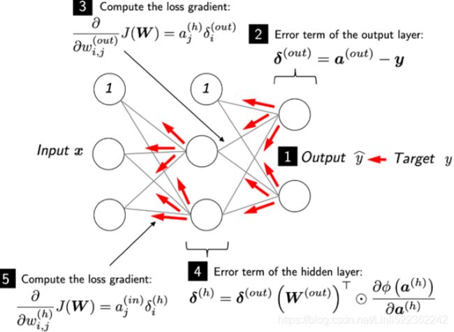
About the convergence in neural networks
You might be wondering why we did not use regular gradient descent but instead used mini-batch learning to train our NN for the handwritten digit classification. You may recall our discussion on SGD that we used to implement online learning. In online learning, we compute the gradient based on a single training example (k =1) at a time to perform the weight update. Although this is a stochastic approach, it often leads to very accurate solutions with a much faster convergence than regular gradient descent. Mini-batch learning is a special form of SGD where we compute the gradient based on a subset k of the n training examples with 1 < k < n. Minibatch learning has the advantage over online learning that we can make use of our vectorized implementations to improve computational efficiency. However, we can update the weights much faster than in regular gradient descent. Intuitively, you can think of mini-batch learning as predicting the voter turnout of a presidential election from a poll by asking only a representative subset of the population rather than asking the entire population (which would be equal to running the actual election).
Multilayer NNs are much harder to train than simpler algorithms such as Adaline, logistic regression, or support vector machines. In multilayer NNs, we typically have hundreds, thousands, or even billions of weights that we need to optimize. Unfortunately, the output function has a rough surface and the optimization algorithm can easily become trapped in local minima, as shown in the following figure:
Note that this representation is extremely simplified since our NN has many dimensions; it makes it impossible to visualize the actual cost surface for the human eye. Here, we only show the cost surface for a single weight on the x-axis. However, the main message is that we do not want our algorithm to get trapped in local minima. By increasing the learning rate, we can more readily escape such local minima. On the other hand, we also increase the chance of overshooting the global optimum if the learning rate is too large. Since we initialize the weights randomly, we start with a solution to the optimization problem that is typically hopelessly wrong.
A few last words about the neural network implementation
You may be wondering why we went through all of this theory just to implement a simple multilayer artificial network that can classify handwritten digits instead of using an open source Python machine learning library. In fact, we will introduce more complex NN models in the next chapters, which we will train using the open source TensorFlow library (https://www.tensorflow.org).
Although the from-scratch implementation in this chapter seems a bit tedious at first, it was a good exercise for understanding the basics behind backpropagation and NN training, and a basic understanding of algorithms is crucial for applying machine learning techniques appropriately and successfully.
Now that you have learned how feedforward NNs work, we are ready to explore more sophisticated DNNs by using TensorFlow, which allows us to construct NNs more efficiently, as we will see in Chapter 13, Parallelizing Neural Network Training with TensorFlow.
Over the past two years, since its release in November 2015, TensorFlow has gained a lot of popularity among machine learning researchers, who use it to construct DNNs because of its ability to optimize mathematical expressions for computations on multidimensional arrays utilizing graphics processing units (GPUs). While TensorFlow can be considered a low-level deep learning library, simplifying APIs such as Keras have been developed that make the construction of common deep learning models even more convenient, which we will see in Chapter 13, Parallelizing Neural Network Training with TensorFlow.
Summary
In this chapter, you have learned the basic concepts behind multilayer artificial NNs, which are currently the hottest topic in machine learning research. In cp2_TrainingSimpleMachineLearningAlgorithmsForClassification_meshgrid_ravel_contourf_OvA_GradientDescent https://blog.csdn.net/Linli522362242/article/details/96429442, we started our journey with simple single-layer NN structures and now we have connected multiple neurons to a powerful NN architecture to solve complex problems such as handwritten digit recognition. We demystified[di:ˈmistifaid]使非神秘化 the popular backpropagation algorithm, which is one of the building blocks of many NN models that are used in deep learning. After learning about the backpropagation algorithm in this chapter, we are well equipped for exploring more complex DNN architectures. In the remaining chapters, we will cover TensorFlow, an open source library geared[gɪəd]连接的 toward deep learning, which allows us to implement and train multilayer NNs more efficiently.