电商数据回归分析
'revenue':用户的下单购买金额 (目标值)
'gender' 性别 1男 0女 空缺 未知
'age' 年龄
'engaged_last_30' 最近30天有关键操作(社区发帖,买家秀)
'lifecycle', 生命周期 A,B,C 注册6个月内 1年内 2年内
' days_since_last_order ' 最近一次下单距今天数 <1说明当天有下单
'previous_order_amount' 以往积累的用户购买金额
'3rd_party_stores' 在非自营店铺购买商品的数量,0说明只在自营店铺购买过
-
缺失值处理
-
性别 可以考虑分成 0 1 未知
-
其它缺失分类特征也可以考虑用上述办法处理
-
年龄 可以用均值,中位数 或者数据模型填充
-
-
可处理成哑变量矩阵的
-
lifecycle
-
-
单变量分析
-
数值类型特征describe
-
-
相关与可视化
-
分析变量之间的相关性
-
-
回归模型
相关API
-
导入数据sn_shop (名字可以任意取)
-
sn_shop.isnull().sum()查看缺失情况
-
fillna() 缺失值填充
-
sn_shop['age'].fillna(sn_shop.age.mean())
-
-
pd.get_dummies(sn_shop) 可以将类别变量转换成one-hot
-
describe()常见统计学指标
-
相关性判断
-
sn_shop.corr()
-
sn_shop.corr()[['revenue']].sort_values('revenue',ascending = False)
-
sns.regplot(x轴变量,y轴变量,数据文件) 进行可视化
-
-
查看模型结果
-
自变量系数 model.coef_
-
截距 model.intercept_
-
-
模型评估
-
score = model.score(x,y) x,y打分
-
predictions = model.predict(x) 计算y预测值
-
error = predictions -y 计算误差
-
rmse = (error** 2).mean() **.5 rmse
-
mae = abs(error).mean() mae
-
import pandas as pd
eshop1=pd.read_csv("ecom.csv")
eshop1.head()
	revenue	gender age	engaged_last_30	lifecycle	days_since_last_order previous_order_amount	3rd_party_stores
0	72.98	1.0	   59.0	    0.0	           B	         4.26	            2343.870	  0
1	200.99	1.0	   51.0	    0.0	           A	         0.94	            8539.872	  0
2	69.98	1.0	   79.0	    0.0	           C	         4.29	            1687.646	  1
3	649.99	NaN	   NaN	    NaN	           C	        14.90	            3498.846	  0
4	83.59	NaN	   NaN	    NaN	           C	        21.13	            3968.490	  4

eshop1.info()

RangeIndex: 29452 entries, 0 to 29451
Data columns (total 8 columns):
 #   Column                   Non-Null Count  Dtype
---  ------                   --------------  -----
 0   revenue                  29452 non-null  float64
 1   gender                   17723 non-null  float64
 2   age                      16716 non-null  float64
 3   engaged_last_30          17723 non-null  float64
 4   lifecycle                29452 non-null  object
 5    days_since_last_order   29452 non-null  float64
 6   previous_order_amount    29452 non-null  float64
 7   3rd_party_stores         29452 non-null  int64
dtypes: float64(6), int64(1), object(1)
memory usage: 1.8+ MB

eshop1.describe()  #revenue出现异常的极大值
| revenue | gender | age | engaged_last_30 | days_since_last_order | previous_order_amount | 3rd_party_stores | |
|---|---|---|---|---|---|---|---|
| count | 29452.000000 | 17723.000000 | 16716.000000 | 17723.000000 | 29452.000000 | 29452.000000 | 29452.000000 |
| mean | 398.288037 | 0.950742 | 60.397404 | 0.073069 | 7.711348 | 2348.904830 | 2.286059 |
| std | 960.251728 | 0.216412 | 14.823026 | 0.260257 | 6.489289 | 2379.774213 | 3.538219 |
| min | 0.020000 | 0.000000 | 18.000000 | 0.000000 | 0.130000 | 0.000000 | 0.000000 |
| 25% | 74.970000 | 1.000000 | 50.000000 | 0.000000 | 2.190000 | 773.506250 | 0.000000 |
| 50% | 175.980000 | 1.000000 | 60.000000 | 0.000000 | 5.970000 | 1655.980000 | 0.000000 |
| 75% | 499.990000 | 1.000000 | 70.000000 | 0.000000 | 11.740000 | 3096.766500 | 3.000000 |
| max | 103466.100000 | 1.000000 | 99.000000 | 1.000000 | 23.710000 | 11597.900000 | 10.000000 |
从年龄age可以看出来大多数是50岁以上的消费者,此消费群体属于中老年群体。消费特征是理性购买,经济实惠,所以整体消费能力不会太高。
eshop1.revenue.quantile(0.995) #分位数计算 说明有百分之99的数值都是低于3000的
显示结果:
3299.79155
175/29452 #平均数
0.005941871519760967
eshop2=eshop1[eshop1["revenue"]<3000]
eshop2.count()
revenue 29262
gender 17623
age 16638
engaged_last_30 17623
lifecycle 29262
days_since_last_order 29262
previous_order_amount 29262
3rd_party_stores 29262
dtype: int64
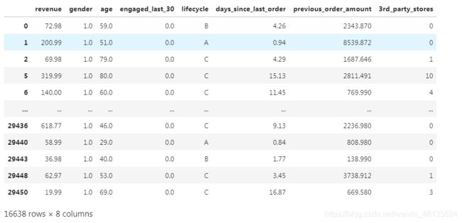
eshop2.dropna().describe() #把缺失值都丢掉 16638个数据
revenue gender age engaged_last_30 days_since_last_order previous_order_amount 3rd_party_stores
count 16638.000000 16638.000000 16638.000000 16638.000000 16638.000000 16638.000000 16638.000000
mean 351.987359 0.956064 60.431843 0.068999 7.254357 2564.011821 1.983051
std 436.813625 0.204958 14.824688 0.253460 6.204628 2469.699088 3.269002
min 0.020000 0.000000 18.000000 0.000000 0.130000 0.000000 0.000000
25% 71.180000 1.000000 50.000000 0.000000 2.100000 901.042500 0.000000
50% 162.980000 1.000000 60.000000 0.000000 5.520000 1846.200500 0.000000
75% 476.712500 1.000000 70.000000 0.000000 11.190000 3378.961750 3.000000
max 2999.800000 1.000000 99.000000 1.000000 23.710000 11597.900000 10.000000
#查看各个值之间的相关性
eshop2.dropna().corr()
显示结果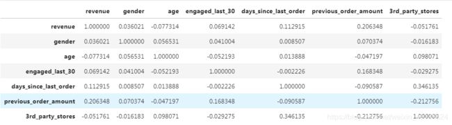
eshop2.dropna().corr()[['revenue']].sort_values('revenue',ascending = False)

	                    revenue
revenue	                1.000000
previous_order_amount	0.206348
days_since_last_order	0.112915
engaged_last_30	        0.069142
gender	                0.036021
3rd_party_stores	   -0.051761
age	                   -0.077314
以上可以发现,由corr得到收入与其他数据之间的相关性,可以发现所有数据对总收入的影响都是弱相关性。0.2以上会出现一点儿相关性,如果到0.3以上有明显的相关性;0.5以上有强相关性。如果显示是弱相关,可视化切记不要选择线型图进行展示。
#设置eshop2作为删除缺失值后的所有值
eshop2.dropna(inplace=True)
eshop2
eshop2 = pd.get_dummies(eshop2)  #把lifecycle进行one_hot转换
eshop2
#显示结果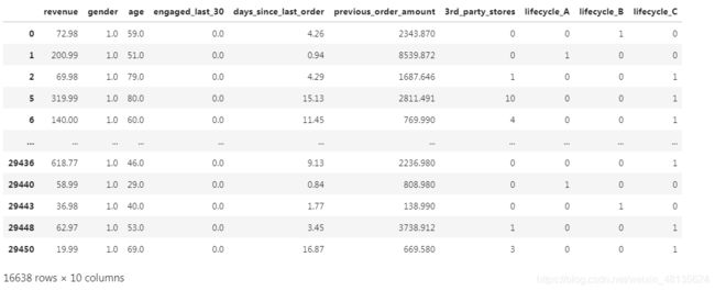
#数据标准化
#from sklearn.preprocessing import StandardScaler
#scaler = StandardScaler()
#x=eshop2[['previous_order_amount']]
#scaler.fit_transform(x)
eshop2["previous_order_amount"]=(eshop2["previous_order_amount"]-eshop2["previous_order_amount"].mean())/eshop2["previous_order_amount"].std()
eshop2["previous_order_amount"]

#from sklearn.preprocessing import scale
#x=pd.DataFrame(scale("这里必须填写框架才可以使用"))

#from sklearn.preprocessing import StandardScaler
#数据标准化
#2.1实例化一个转换器
#transfer=StandardScaler()
#1.2 调用fit transform方法
#minmax_data=transfer.fit_transform(data[['1','2','3']])
#print("最小值最大值归一化处理的结果:\n", minmax_data)
eshop2.previous_order_amount
#显示结果
0 -0.002116
1 2.601494
2 -0.277866
3 0.483214
4 0.680563
...
29447 -0.757939
29448 0.584092
29449 -0.449360
29450 -0.705666
29451 -0.103352
Name: previous_order_amount, Length: 29452, dtype: float64对用户的下单总金额进行分组:
pd.cut(eshop2['revenue'],[0,10,75,176,500,1000,3000]).value_counts()
(10, 75]        4336
(176, 500]      4217
(75, 176]       4133
(500, 1000]     2496
(1000, 3000]    1383
(0, 10]           73
Name: revenue, dtype: int64
由上边可以看出用户的下单购买金额比较少的人数占比大。大部分都在175以下.消费能力低。
不同年龄段在所有年龄中的分布:
bins=[0,50,60,70,100]
eshop2['Age_range']=pd.cut(eshop2.age,bins,right=False)
eshop2.groupby(['Age_range'])['age'].describe()
#显示结果

              count	   mean	       std	     min	25%	     50%	75%  	max
Age_range
[0, 50)	    3994.0	41.533050	6.398882	18.0	38.0	43.0	47.0	49.0
[50, 60)	4140.0	54.579227	2.863615	50.0	52.0	55.0	57.0	59.0
[60, 70)	4022.0	64.384137	2.851611	60.0	62.0	64.0	67.0	69.0
[70, 100)	4482.0	79.132307	7.127877	70.0	73.0	78.0	84.0	99.0
#可视化分析
import seaborn as sns
import matplotlib.pyplot as plt
%matplotlib inline
#%matplotlib inline 可以在Ipython编译器里直接使用,功能是可以内嵌绘图,并且可以省略掉plt.show()这一步。
#线性关系可视化
#斜率与相关系数有关;sns.regplot():绘图数据和线性回归模型拟合
sns.barplot(x="Age_range",y="revenue",data=eshop2)
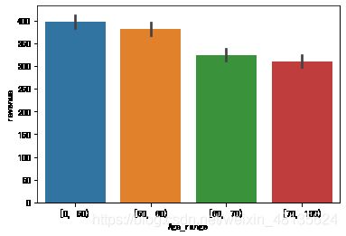
由上图可知,年轻人消费人数较少,但是占总收入相比较高。年轻人更注重时尚,对价格不敏感。更多的消费人群分布在50岁到100岁之间。