Python-统计学应用-回归分析

import pandas as pd
import statsmodels.api as sm
import matplotlib.pyplot as plt
import numpy as np

一元线性回归

拟合线性模型主要通过statsmodels包中的OLS类完成

1. fit()——得到线性回归的结果
2. summary()——看出拟合模型的详细结果
3. params()——列入拟合模型的参数
4. conf_int()——提供模型参数的置信区间
5. fittedvalues——模型的拟合值
6. resid——模型的残差值
7. aic——赤池信息统计量
8. predict()——用拟合模型对新的数据集预测解释变量

trd_index = pd.read_table('TRD_Index.txt', sep='\t')
sh_index = trd_index[trd_index.Indexcd == 1]
sz_index = trd_index[trd_index.Indexcd == 399106]
sh_ret = sh_index.Retindex
sz_ret = sz_index.Retindex
sh_ret.index = sz_ret.index

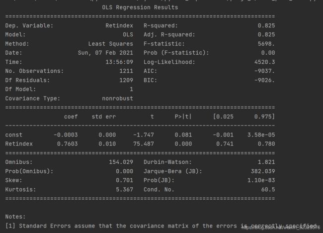
model = sm.OLS(sh_ret, sm.add_constant(sz_ret)).fit()
print(model.summary())

结果：

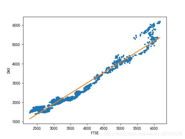
绘制拟合曲线

model = sm.OLS(eu_stock_market.DAX, sm.add_constant(eu_stock_market.FTSE)).fit()
print(model.summary())
plt.plot(eu_stock_market.FTSE, eu_stock_market.DAX, '.',
         eu_stock_market.FTSE, model.fittedvalues, '-')
plt.xlabel('FTSE')
plt.ylabel('DAX')
plt.show()

模型检验

1. 线性：若因变量与自变量线性相关，残差值应该和拟合值没有任何的系统关联，呈现出围绕0随机分布的状态。

plt.scatter(model.fittedvalues, model.resid)
plt.xlabel('fitted_values')
plt.ylabel('resid')
plt.show()

基本满足该假设。

2. 正态性：当因变量呈正态分布时，模型的残差项应该是一个均值为0的正态分布。
   [正态Q-Q图是在正态分布对应的值下，标准化残差的概率图，若满足正态性假设，那么图上的点应该落在一条直线上，若不是，则违背了正态性的假设]

sm.qqplot(model.resid_pearson, stats.norm, line='45')
plt.show()

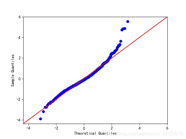
*残差在两端出现了较为严重的偏离，数据可能不满足正态性假设。

3. 同方差性：若满足不变方差假设，那么再位置尺度图上，各点分布应该呈现出一条水平的宽度一致的条带形状。

plt.scatter(model.fittedvalues,model.resid_pearson**0.5)
plt.xlabel('fitted_values')
plt.ylabel('square root of standardized residuals')
plt.show()

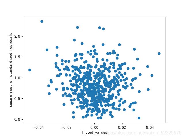
基本满足该假设。

多元线性回归

penn = pd.read_csv('Penn World Table——1.csv')
model = sm.OLS(np.log(penn.rgdpe), sm.add_constant(penn.iloc[:, -6:])).fit()
print(model.summary())

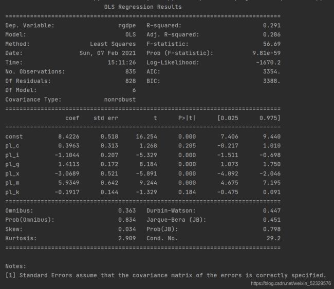
其中pl_c, pl_k不显著。

自变量共线性因素的新模型

print(penn.iloc[:, -6:].corr())

# 结果

#           pl_c      pl_i      pl_g      pl_x      pl_m      pl_k
# pl_c  1.000000  0.718931  0.636698  0.078841  0.213328  0.553757
# pl_i  0.718931  1.000000  0.259183  0.072019  0.139333  0.779306
# pl_g  0.636698  0.259183  1.000000  0.130729  0.256069  0.211259
# pl_x  0.078841  0.072019  0.130729  1.000000  0.477304 -0.065623
# pl_m  0.213328  0.139333  0.256069  0.477304  1.000000  0.000531
# pl_k  0.553757  0.779306  0.211259 -0.065623  0.000531  1.000000

可以看出，pl_c和多个变量之间存在较强的相关性且pl_k和pl_i的相关系数也较大。
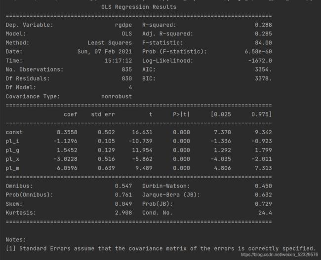
优化模型为：

model = sm.OLS(np.log(penn.rgdpe), sm.add_constant(penn.iloc[:, -5:-1])).fit()
print(model.summary())

示例

Y = b0 + b1X + b2X **2 + ε , ε~N(0, δ **2)

x = [20, 25, 30, 35, 40, 50, 60, 65, 70, 75, 80, 90]
y = [1.81, 1.7, 1.65, 1.55, 1.48, 1.4, 1.3, 1.26, 1.24, 1.21, 1.2, 1.18]
plt.scatter(x, y)
plt.show()

independent = np.array([x, [i ** 2 for i in x]]).T
model = sm.OLS(y, sm.add_constant(independent)).fit()
print(model.summary())
print(model.predict(np.array([1, 95, 95 ** 2])).T)

当ethnicity的数据非数值时:

import statsmodels.formula.api as smf

cps = pd.read_csv('CPS1988.csv')
model = smf.ols('np.log(wage)~experience+education+ethnicity',
                data=cps).fit()
print(model.summary())
model2 = smf.ols('np.log(wage)~experience+np.power(experience,2)+education+ethnicity',
                 data=cps).fit()
print(model2.summary())