Linear Regression

Reference:

Bishop C M. Pattern recognition and machine learning[M]. springer, 2006.

- Chapter 1 up to and including Subsection 1.2.5
- Chapter 3 up to and including 3.1.2

Linear Regression: Intro

Example: Polynomial Curve Fitting

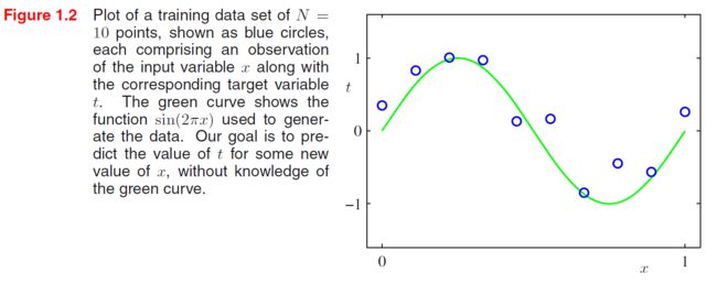
Suppose that we are given a training set comprising $N$ observations of $x$, written $\mathbf{X}=(x^{(1)},\cdots ,x^{(N)}{)}^T$, together with corresponding observations of the values of $t$, denoted $\mathbf{t}=(t^{(1)},\cdots ,t^{(N)}{)}^T$. Our goal is to exploit this training set in order to make predictions of the value of $\hat{t}$ of the target variable for some new value $\hat{x}$ of the input variable.

For this moment, we shall fit the data using a polynomial function of the form
$$y(x,\mathbf{w})=w_0+w_{1}x+\cdots +w_M{x}^M=\sum _{j=0}^M{w}_j{x}^j\text{\hspace{1em}(CF.1)}$$
where $M$ is the order of the polynomial. Note that, although the polynomial function $y(x,\mathbf{w})$ is a nonlinear function of $x$, it is a linear function of the coefficients $\mathbf{w}$. Functions, such as the polynomial, which are linear in the unknown parameters have important properties and are called linear models.

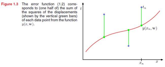
The values of the coefficients will be determined by fitting the polynomial to the training data. This can be done by minimizing an error function that measures the misfit between the function $y(x,\mathbf{w})$. One simple choice of error function, is given by the sum of the squares of the errors between the predictions $y(x^{(n)},\mathbf{w})$ for each data point $x^{(n)}$ and the corresponding target values $t^{(n)}$, so that we minimize
$$E(\mathbf{w})=\frac{1}{2}\sum _{n=1}^N\{y(x^{(n)},\mathbf{w})-t^{(n)}{\}}^2\text{\hspace{1em}(CF.2)}$$
where the factor of $1/2$ is included for later convenience.

We can solve the curve fitting problem by setting the derivative of $E(\mathbf{w})$ w.r.t. $\mathbf{w}$ equal to zero. Because the error function is a quadratic function of the coefficients $\mathbf{w}$, its derivatives with respect to the coefficients will be linear in the elements of $ \mathbf w$, and so the minimization of the error function has a unique solution, denoted by ${\mathbf{w}}^{\ast }$, which can be found in closed form. The resulting polynomial is given by the function $y(x,{\mathbf{w}}^{\ast })$.

There remains the problem of choosing the order $M$ of the polynomial. In Figure 1.4, we show four examples of the results of fitting polynomials having orders $M=0,1,3,9$ to the data set shown in Figure 1.2.

We notice that the constant $(M=0)$ and first order $(M=1)$ polynomials give rather poor fits to the data and consequently rather poor representations of the function $sin(2\pi x)$. The third order $(M=3)$ polynomial seems to give the best fit to the function $sin(2\pi x)$ of the examples shown in Figure 1.4. When we go to a much higher order polynomial $(M=9)$, we obtain an excellent fit to the training data since this polynomial contains $10$ degrees of freedom corresponding to the $10$ coefficients $w_0,\cdots ,w_9$. In fact, the polynomial passes exactly through each data point and $E({\mathbf{w}}^{\ast })=0$. However, the fitted curve oscillates wildly and gives a very poor representation of the function $sin(2\pi x)$. This latter behavior is known as overfitting.

We shall see that the least squares approach to finding the model parameters represents a specific case of maximum likelihood, and that the over-fitting problem can be understood as a general property of maximum likelihood.

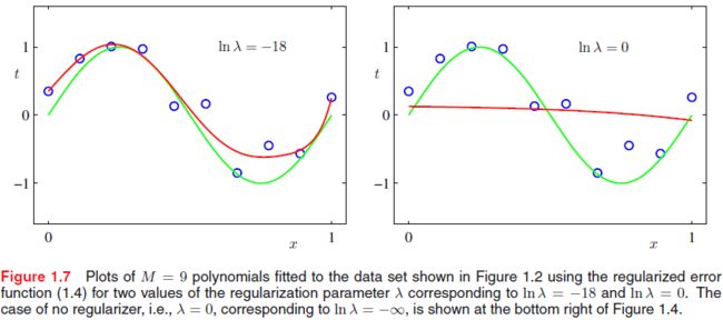
One technique that is often used to control the over-fitting phenomenon in such cases is that of regularization, which involves adding a penalty term to the error function in order to discourage the coefficients from reaching large values. The simplest such penalty term takes the form of a sum of squares of all of the coefficients, leading to a modified error function of the form
$$\tilde{E}(\mathbf{w})=\frac{1}{2}\sum _{n=1}^N\{y(x^{(n)},\mathbf{w})-t^{(n)}{\}}^2+\frac{\lambda }{2}\Vert \mathbf{w}{\Vert }^2\text{\hspace{1em}(CF.3)}$$
where the $\lambda$ governs the relative importance of the regularization term compared with the sum-of-squares error term.

Probabilistic Perspective

We have seen how the problem of polynomial curve fitting can be expressed in terms of error minimization. Here we return to the curve fitting example and view it from a probabilistic perspective, thereby gaining some insights into error functions and regularization, as well as taking us towards a full Bayesian treatment.

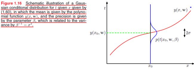
We assume that, given the value of $x$, the corresponding value of $t$ has a Gaussian distribution with a mean equal to the value $y(x,\mathbf{w})$ of the polynomial curve given by $(CF.1)$. Thus we have
$$p(t|x,\mathbf{w},\beta )=\mathcal{N}(t|y(x,\mathbf{w}),{\beta }^{-1})\text{\hspace{1em}(PP.1)}$$
where we have defined a precision parameter $\beta$ corresponding to the inverse variance of the distribution.

We now use the training data $(\mathbf{X},\mathbf{t})$ to determine the value of the unknown parameters $\mathbf{w}$ and $\beta$ by maximum likelihood. If the data are assumed to be drawn independently from the distribution $(PP.1)$, then the likelihood function is given by
$$p(\mathbf{t}|\mathbf{X},\mathbf{w},\beta )=\prod _{n=1}^N\mathcal{N}(t^{(n)}|y(x^{(n)},\mathbf{w}),{\beta }^{-1})\text{\hspace{1em}(PP.2)}$$
It is convenient to maximize the logarithm of the likelihood function.
$$\ln p(\mathbf{t}|\mathbf{X},\mathbf{w},\beta )=-\frac{\beta }{2}\sum _{n=1}^N\{y(x^{(n)},\mathbf{w})-t^{(n)}{\}}^2+\frac{N}{2}\ln \beta -\frac{N}{2}\ln (2\pi )\text{\hspace{1em}(PP.3)}$$
We therefore see that maximizing likelihood is equivalent, so far as determining $\mathbf{w}$ is concerned, to minimizing the sum-of-squares error function defined by $(CF.2)$.
$$E(\mathbf{w})=\frac{1}{2}\sum _{n=1}^N\{y(x^{(n)},\mathbf{w})-t^{(n)}{\}}^2\text{\hspace{1em}(CF.2)}$$
The optimized value is denoted as ${\mathbf{w}}_{ML}$.

We can also use maximum likelihood to determine the precision parameter $\beta$ of the Gaussian conditional distribution. Maximizing $(PP.3)$ w.r.t. $\beta$ gives
$$\frac{1}{{\beta }_{ML}}=\frac{1}{N}\sum _{n=1}^N\{y(x^{(n)},\mathbf{w})-t^{(n)}{\}}^2\text{\hspace{1em}(PP.4)}$$
Note that the solution for ${\mathbf{w}}_{ML}$ decouples from that for $\beta$, so we can first evaluate $(CF.2)$ and subsequently use this result to evaluate $(PP.4)$.

Having determined the parameters $\mathbf{w}$ and $\beta$, we can now make predictions for new values of $x$. Because we now have a probabilistic model, these are expressed in terms of the predictive distribution that gives the probability distribution over t, rather than simply a point estimate, and is obtained by substituting the maximum likelihood parameters into $(PP.1)$ to give
$$p(t|x,{\mathbf{w}}_{ML},{\beta }_{ML})=\mathcal{N}(t|y(x,{\mathbf{w}}_{ML}),{\beta }_{ML}^{-1})\text{\hspace{1em}(PP.5)}$$
Now let us take a step towards a more Bayesian approach and introduce a prior distribution over the polynomial coefficients $\mathbf{w}$. For simplicity, let us consider a Gaussian distribution of the form
$$p(\mathbf{w}|\alpha )=\mathcal{N}(\mathbf{w}|0,{\alpha }^{-1}\mathbf{I})={\left(\frac{\alpha }{2\pi }\right)}^{(M+1)/2}\exp \left\{-\frac{\alpha }{2}{\mathbf{w}}^T\mathbf{w}\right\}\text{\hspace{1em}(PP.6)}$$
where $\alpha$ is the precision of the distribution, and $(M+1)$ is the total number of elements in the vector $\mathbf{w}$ for an $M^{th}$ order polynomial.

Using Bayes’ theorem, the posterior distribution for $\mathbf{w}$ is proportional to the product of the prior distribution and the likelihood function
$$p(\mathbf{w}|\mathbf{X},\mathbf{t},\alpha ,\beta )\propto p(\mathbf{t}|\mathbf{X},\mathbf{w},\beta )p(\mathbf{w}|\alpha )\text{\hspace{1em}(PP.7)}$$
We can now determine w by finding the most probable value of $\mathbf{w}$ given the data, in other words by maximizing the posterior distribution. This technique is called maximum posterior, or simply MAP. Taking the negative logarithm of $(PP.7)$ and combining with $(PP.3)$ and $(PP.6)$, we find that the maximum of the posterior is given by the minimum of
$$\frac{\beta }{2}\sum _{n=1}^N\{y(x^{(n)},\mathbf{w})-t^{(n)}{\}}^2+\frac{\alpha }{2}{\mathbf{w}}^T\mathbf{w}\text{\hspace{1em}(PP.8)}$$
Thus we see that maximizing the posterior distribution is equivalent to minimizing the regularized sum-of-squares error function encountered earlier in the form $(CF.3)$, with a regularization parameter given by $\lambda =\alpha /\beta$.

Linear Basis Function Models

The simplest linear model for regression involves a linear combination of the input variables
$$y(\mathbf{x},\mathbf{w})=w_0+w_1{x}_1+\cdots w_D{x}_D\text{\hspace{1em}(LM.1)}$$
where $\mathbf{x}=[x_1,x_2,\cdots ,x_D{]}^T$ are the features. This is often simply known as linear regression. However, a linear function of the input variables $x_i$ imposes significant limitations on the model. We therefore extend the class of models by considering linear combinations of fixed nonlinear functions of the input variables of the form
$$y(\mathbf{x},\mathbf{w})=w_0+\sum _{j=1}^{M-1}{w}_j{\varphi }_j(\mathbf{x})\text{\hspace{1em}(LM.2)}$$
where ${\varphi }_j(\mathbf{x})$ are known as basis functions.

It is often convenient to define an additional dummy ‘basis function’ ${\varphi }_0(\mathbf{x})=1$ so that
$$y(\mathbf{x},\mathbf{w})=\sum _{j=0}^{M-1}{w}_j{\varphi }_j(\mathbf{x})={\mathbf{w}}^T\varphi (\mathbf{x})\text{\hspace{1em}(LM.3)}$$
By using nonlinear basis functions, we allow the function $y(\mathbf{x},\mathbf{w})$ to be a nonlinear function of the input vector $\mathbf{x}$. Functions of the form $(LM.3)$ are called linear models, however, because this function is linear in $\mathbf{w}$.

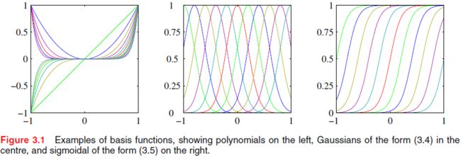
In the [curve fitting example](# Example: Polynomial Curve Fitting), the basis functions take the form of powers of $x$ so that ${\varphi }_j(x)=x^j$. There are many other possible choices for the basis functions, for example
$$\text{Gaussian basis functions: }{\varphi }_j(x)=\exp \left\{-\frac{(x-{\mu }_j{)}^2}{2s^2}\right\}$$

$$\begin{gathered} \text{Sigmoidal basis functions: }{\varphi }_j(x)=\sigma \left(\frac{x-{\mu }_j}{s}\right) \\ \text{ where }\sigma (a)\text{ is the sigmoid function defined by }\sigma (a)=\frac{1}{1+\exp (-a)} \end{gathered}$$

Most of the discussion, however, is independent of the particular choice of basis function set, and so for most of our discussion we shall not specify the particular form of the basis functions.

Maximum likelihood and least squares

In [Probabilistic Perspective](# Probabilistic Perspective), we showed that the error function could be motivated as the maximum likelihood solution under the assumed Gaussian noise model. Let us return to this discussion and consider the least squares approach, and its relation to maximum likelihood, in more detail.

As before, we assume that the target variable $t$ is given by a deterministic function $y(\mathbf{x},\mathbf{w})$ with additive Gaussian noise so that
$$t=y(\mathbf{x},\mathbf{w})+ϵ\text{\hspace{1em}(LM.4)}$$
where $ϵ$ is a zero mean Gaussian random variable with precision $\beta$. Thus we can write
$$p(t|\mathbf{x},\mathbf{w},\beta )=\mathcal{N}(t|y(\mathbf{x},\mathbf{w}),{\beta }^{-1})\text{\hspace{1em}(LM.5)}$$
Now consider a data set of inputs $\mathbf{X}=\{{\mathbf{x}}^{(1)},\cdots ,{\mathbf{x}}^{(N)}\}$ with corresponding target values $\mathbf{t}=[t^{(1)},\cdots ,t^{(N)}]$. Making the assumption that these data points are drawn independently from the distribution $(LM.5)$, we obtain the following expression for the likelihood function, which is a function of the adjustable parameters $\mathbf{w}$ and $\beta$, in the form
$$p(\mathbf{t}|\mathbf{X},\mathbf{w},\beta )=\prod _{n=1}^N\mathcal{N}(t^{(n)}|{\mathbf{w}}^T\varphi ({\mathbf{x}}^{(n)}),{\beta }^{-1})\text{\hspace{1em}(LM.6)}$$
Since $\mathbf{X}$ always appear in the set of conditioning variables, we will drop the explicit $\mathbf{X}$ from expressions for conciseness. Taking the logarithm of the likelihood function, we have
$$\begin{array}{rl}\ln p(\mathbf{t}|\mathbf{w},\beta )& =\sum _{n=1}^N\ln \mathcal{N}\left(t^{(n)}|{\mathbf{w}}^{\mathrm{T}}\varphi \left({\mathbf{x}}^{(n)}\right),{\beta }^{-1}\right)\\ & =\frac{N}{2}\ln \beta -\frac{N}{2}\ln (2\pi )-\beta E_D(\mathbf{w})\end{array}\text{\hspace{1em}(LM.7)}$$
where the sum-of-squares error function is defined by
$$E_D(\mathbf{w})=\frac{1}{2}\sum _{n=1}^N{\left\{t^{(n)}-{\mathbf{w}}^{\mathrm{T}}\varphi \left({\mathbf{x}}^{(n)}\right)\right\}}^2\text{\hspace{1em}(LM.8)}$$
We see that maximization of the likelihood function under a conditional Gaussian noise distribution for a linear model is equivalent to minimizing a sum-of-squares error function given by $E_D(\mathbf{w})$.

Consider first the maximization with respect to $\mathbf{w}$. The gradient of the log likelihood function $(LM.7)$ takes the form
$$\nabla \ln p(\mathbf{t}|\mathbf{w},\beta )=\sum _{n=1}^N\left\{t^{(n)}-{\mathbf{w}}^{\mathrm{T}}\varphi \left({\mathbf{x}}^{(n)}\right)\right\}\varphi ({\mathbf{x}}^{(n)}{)}^{\mathrm{T}}\text{\hspace{1em}(LM.9)}$$
Setting this gradient to zero gives
$$\sum _{n=1}^N{t}^{(n)}\varphi ({\mathbf{x}}^{(n)}{)}^{\mathrm{T}}-{\mathbf{w}}^{\mathrm{T}}\left(\sum _{n=1}^N\varphi \left({\mathbf{x}}^{(n)}\right)\varphi ({\mathbf{x}}^{(n)}{)}^{\mathrm{T}}\right)=0\text{\hspace{1em}(LM.10)}$$
Solving for $\mathbf{w}$ we obtain
$${\mathbf{w}}_{ML}=({\mathbf{\Phi }}^T\mathbf{\Phi }{)}^{-1}{\mathbf{\Phi }}^T\mathbf{t}\triangleq {\mathbf{\Phi }}^{†}\mathbf{t}\text{\hspace{1em}(LM.11)}$$
where
$$\mathbf{\Phi }=\left[\begin{array}{c}\varphi ({\mathbf{x}}^{(1)}{)}^T\\ ⋮\\ \varphi ({\mathbf{x}}^{(N)}{)}^T\end{array}\right]=\left[\begin{array}{ccc}\varphi (x_1^{(1)})& \cdots & \varphi (x_D^{(1)})\\ ⋮& \ddots & ⋮\\ \varphi (x_1^{(N)})& \cdots & \varphi (x_D^{(N)})\end{array}\right]\text{\hspace{1em}(LM.12)}$$
which are known as the normal equations for the least square problem.

Then we can also maximize the log likelihood function $(LM.7)$ with respect to the noise precision parameter $\beta$, giving
$$\frac{1}{{\beta }_{ML}}=\frac{1}{N}\sum _{n=1}^N{\left\{t^{(n)}-{\mathbf{w}}_{ML}^{\mathrm{T}}\varphi \left({\mathbf{x}}^{(n)}\right)\right\}}^2$$
and so we see that the inverse of the noise precision is given by the residual variance of the target values around the regression function.

Geometry of least squares

We can stack $y(\mathbf{x},\mathbf{w})$ as a vector with the definition in $(LM.12)$
$$\mathbf{y}=\left[\begin{array}{c}{y}^{(1)}({\mathbf{x}}^{(1)},\mathbf{w})\\ ⋮\\ y^{(N)}({\mathbf{x}}^{(N)},\mathbf{w})\end{array}\right]=\left[\begin{array}{c}\varphi ({\mathbf{x}}^{(1)}{)}^T\\ ⋮\\ \varphi ({\mathbf{x}}^{(N)}{)}^T\end{array}\right]\mathbf{w}=\mathbf{\Phi }\mathbf{w}\text{\hspace{1em}(LM.13)}$$
Then minimize the error function $(LM.8)$ is equivalent to minimize
$$E(\mathbf{w})=\Vert \mathbf{\Phi }\mathbf{w}-\mathbf{t}{\Vert }_2\text{\hspace{1em}(LM.14)}$$
If the number of features $D$ is smaller than the number of data points $N$, the columns of $\mathbf{\Phi }$, denoted as ${\phi }_j,j=1,\cdots ,D$ will span a linear subspace $\mathcal{S}$ of dimensionality $D$. $\mathbf{y}$ will be an arbitrary linear combination of the vectors ${\phi }_j$, thus can live anywhere in the $D$-dimensional subspace. $(LM.14)$ is then equal to the Euclidean distance between $\mathbf{y}$ and $\mathbf{t}$. Therefore, $\mathbf{y}$ is the orthogonal projection of $\mathbf{t}$ onto the subspace $\mathcal{S}$, i.e.,
$$(\mathbf{t}-\mathbf{\Phi }\mathbf{w})\in {\mathcal{S}}^{\perp }⟹{\mathbf{\Phi }}^T(\mathbf{\Phi }\mathbf{w}-\mathbf{t})=0\text{\hspace{1em}(LM.15)}$$