R数据科学 R for data sciences

《R数据科学》的再次回顾学习，以及使用tidyverse过程中的一些new tricks学习记录。

[TOC]

前言

reprex包：创建简单的可重现实例。检查问题所在。

一使用ggplot2进行数据可视化

坐标系ggplot()，在此函数种添加的映射会作为全局变量应用到图中的每个几何对象种。
图层geom_point点图层
映射数据为图形属性 mapping=aes()，要想将图形属性映射为变量，需要在函数aes()中将图形属性的名称和变量的名称关联起来。
标度变化：将变量（数据）分配唯一的图形属性水平。
手动设置图形属性，此是在geom_point()层面。此时，这个颜色是不会传达变量数据的信息。
分层facet：facet_grid()可以通过两个变量对图分层`facet_grid(drv_cyl)或(.cyl)
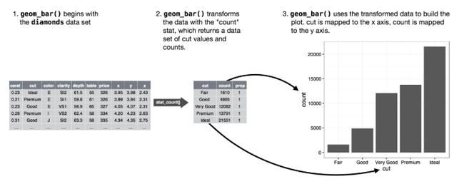
分组aes(group)此种按照图形属性的分组不用添加图例，也不用为几何对象添加区分特征
统计变换：绘图时用来计算新数据的算法称为stat(statistical transformation,统计变化)。比如对于geom_bar()默认是只对一个数据x映射，其统计变化后生成数据x种的每个值的count数。
- 每个几何对象函数都有一个默认的统计变换，每个统计变换函数都有一个默认的几何对象。
- 如需要展示二维柱状图数据，geom_bar(mapping=aes(x=a,y=b),stat="identity ")

image

图形属性/位置调整：
- color,fill
- 位置调整参数position有三个选项："identity","fill","dodge"
- position="dodge"参数可分组显示数据，将每组种的条形依次并列放置，可以轻松比较每个条形表示的具体数值。
  
  image
- 数据的聚集模式无法很好确定，因为存在数据的过绘制问题（很多彼此十分近的点重叠了）position="jitter"对于geom_position()函数来说，jitter的位置方式为抖动会排除过绘制问题ggplot(data = mpg) + geom_point(mapping = aes(x = displ, y = hwy), position = "jitter")
坐标系：
- coord_flip()函数可以交换x轴和y轴
  
  image
- labs()：modify axis, legend, and plot labels.
- coord_polar()极坐标
  
  image

mpg
str(mpg)
data<- mpg
?mpg ##查看mpg数据的说明
ggplot(data = mpg)+geom_point(aes(x=displ,y=hwy))

ggplot(mpg)+geom_point(mapping = aes(x=displ,y=hwy,color=class),color="#EF5C4E",shape=19)
ggplot(mpg)+geom_point(mapping = aes(x=displ,y=hwy),color="#EF5C4E",shape=19)
ggplot(mpg)+geom_point(mapping = aes(x=displ,y=hwy,stroke=displ),shape=19)
## 添加两个图层：geom_point,geom_smooth()
ggplot(mpg)+geom_point(mapping = aes(x=displ,y=hwy,color=drv))+geom_smooth(mapping = aes(x=displ,y=hwy,linetype=drv,color=drv))
# 添加分组
ggplot(data = mpg)+geom_smooth(mapping = aes(x=displ,y=hwy,group=drv))
ggplot(data = mpg)+geom_smooth(mapping = aes(x=displ,y=hwy,color=drv),show.legend = F) ## 图例 show.legend=F

## 在不同的图层中添加指定不同的数据
## data=filter(mpg,class=="suv"), se=F，表示去除f波动的范围。
ggplot(data = mpg,mapping = aes(x=displ,y=hwy))+geom_point(mapping = aes(color=class))+geom_smooth(data = filter(.data = mpg,class=="suv"))

##exercices
ggplot(data = mpg,mapping = aes(x=displ,y=hwy))+geom_point()+geom_smooth(se = F)
ggplot(data = mpg,mapping = aes(x=displ,y=hwy))+geom_point()+geom_smooth(se = F,mapping = aes(group=drv))
ggplot(data = mpg,mapping = aes(x=displ,y=hwy,color=drv))+geom_point()+geom_smooth(se = F)
ggplot(data = mpg,mapping = aes(x=displ,y=hwy))+geom_point(mapping = aes(color=drv))+geom_smooth(se = F)
ggplot(data = mpg,mapping = aes(x=displ,y=hwy))+geom_point(mapping = aes(color=drv))+geom_smooth(mapping = aes(linetype=drv),se = F)
ggplot(data = mpg,mapping = aes(x=displ,y=hwy))+geom_point(mapping = aes(color=drv))

### 统计变换
ggplot(data = mpg,mapping = aes(x=displ,y=hwy))+geom_point()+geom_smooth(se = F)
ggplot(data=diamonds)+stat_summary(mapping = aes(x=cut,y=depth))
ggplot(data=diamonds)+geom_boxplot(mapping = aes(x=cut,y=price))
ggplot(data=diamonds)+geom_bar(mapping = aes(x=cut))
ggplot(data=diamonds)+geom_bar(mapping = aes(x=cut,y=..prop..),group=2)

### 图形调整,位置调整
ggplot(diamonds)+geom_bar(mapping = aes(x=cut,fill=cut),color="black")+scale_fill_brewer(palette = "Set3")
ggplot(diamonds)+geom_bar(mapping = aes(x=cut,fill=clarity))+scale_fill_brewer(palette = "Set2")
ggplot(diamonds)+geom_bar(mapping=aes(x=cut,color=clarity),position = "dodge")+scale_fill_brewer(palette = "Set2")
ggplot(mpg)+geom_point(mapping = aes(x=displ,y=hwy),position = "jitter")
##exercises
ggplot(mpg,mapping = aes(x=cty,y=hwy))+geom_point(position = "jitter")+geom_smooth(color="black")
ggplot(mpg,mapping = aes(x=cty,y=hwy))+geom_jitter()
ggplot(mpg,mapping = aes(x=cty,y=hwy))+geom_count()
ggplot(mpg)+geom_boxplot(mapping = aes(x=manufacturer,y=hwy),position = "identity")
?geom_boxplot

###1.9 坐标系
ggplot(mpg,mapping = aes(x=class,y=hwy))+geom_boxplot()+coord_flip()
nz <- map_data("nz")
?map_data
ggplot(data=diamonds)+geom_bar(mapping = aes(x=cut,fill=cut),show.legend = FALSE)+theme(aspect.ratio = 1)+labs()
bar+scale_color_brewer(palette = "Set2")
bar+coord_flip()
bar+coord_polar()

二工作流：基础 Workflow：basics

赋值：小技巧，alt+减号会自动输入赋值符号<- 并在前后加空格
对象：用snake_case命名法小写字母，以_分割。
Rstudio中快捷查看命令：Alt+Shift+K

三使用dplyr进行数据转换

特殊的data.frametibble。
变量variable类型：
- int：
- dbl(num的一种？):双精度浮点数变量，或称实数。
- chr：字符向量/字符串
- dttm：日期+时间
- lgl：逻辑型变量
- fctr（factor）：因子
- date：日期型变量
基础函数：filter(),arrange(),select(),mutate(),summarize(),group_by()
使用filter()筛选:
- filter(flights, arr_delay<=10).
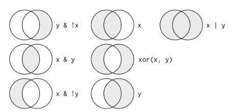
- 比较运算符 ==, !=, <=
- 逻辑运算符 x & !y, x|y, xor(x,y)
  
  image
- 缺失值 NA, is.na()
- %in% ：month %in% c(11, 12)
- distinct(iris, Species)删除重复行
- sample_n()任意挑选行
- slice(irsi,10:15)

## filter()
(jan1 <- filter(flights,month==1,day==1))
(dec25 <- filter(flights,month==12,day==25))
filter(flights,month>=11)
(nov_dec <- filter(flights,month %in% c(11,12)))
filter(flights,!(arr_delay<=120 | dep_delay<=120))
NA>=10
x <- NA
is.na(x)
df <- tibble(x=c(1,NA,2))
filter(df,x>1)
filter(df,is.na(x)|x>1)
### exercise
filter(flights,carrier %in% c("UA","AA","DL"))
filter(flights,month %in% c(7,8,9))
filter(flights,arr_delay>120 & dep_delay==0)
filter(flights,dep_delay >= 60 & (dep_delay-arr_delay>=30)) 
filter(flights,dep_time ==2400| dep_time<=600)
filter(flights,is.na(dep_time))

使用 arrange()按照列(variable)的值values进行排序
- desc倒序
- 缺失值排在最后，若想提前可desc(is.na())
- top_n(10,wind)选择wind变量从大到小的前10个。

# arrange()
arrange(flights,desc(dep_delay,arr_delay)) #降序排列
arrange(flights,desc(is.na(dep_delay),arr_delay)) ##将NA值排列到前面

### find the 5 cars with highest hp without ordering them
mtcars %>% top_n(5, hp)

使用select()选择列：（数据集会有成千上万个变量，select选出变量的子集）
- 选出year~day之间的列：select(flights, year:day)
- 选出排除year~day列：select(flights,-(year:dat))
- 匹配变量中的名称： matches(""), contains("ijk")
- 匹配变量中的开头，结尾名称starts_with(""), ends_with(),
- rename()对列变量重新命名
- everything()辅助函数来将某几列提前。

## select()
select(flights,year:day)
select(flights,-(year:day)) ## 不包括year:day
select(flights,starts_with("s"))
select(flights,ends_with("e"))
select(flights,matches("time"))
select(flights,matches("(.)\\1"))

rename(flights,tail_num=tailnum) ##对变量进行重命名
select(flights,-(month:day),everything()) ## 结合everything()辅助函数 对某几列提前, 置后同理
select(flights, hour:time_hour,everything())
###exercise
select(flights,year,year,year)
select(flights,one_of(c("year","month","day","dep_delay")))
select(flights,contains("TIME"))

使用mutate()添加新的列/变量：
- mutate() 新列添加到已有列的后面；
- transmute 只保留新的变量。
- 常用的运算符号：求整%/%，求余%%，偏移函数lead(), lag()，累加和和滚动聚合，逻辑比较，排秩。
- ==rename()== 可对变量名称进行重新命名。
- ==rename_all(~str_replace(., "", ""))== 可以根据正则匹配进行改名。
- ==mutate_all()== 可对所有observations进行修改。
- ==case_when()== 根据已有的columns创建新的discrete variables。

# mutate() 在tibble后 添加新变量/列
flights_sml <- select(flights,year:day,matches("_delay"),distance,air_time)
flights_sml
mutate(flights_sml,flying_delay=arr_delay-dep_delay,speed=distance/air_time * 60 )
flights_sml
transmute(flights,gain=arr_delay-dep_delay,hour=air_time/60,gain_per_hour=gain/hour)

mutate(flights,dep_time=((dep_time%/%100 * 60)+(dep_time%%100))) ## 会直接在flights中改动dep_time
flights
transmute(flights,air_time,duration=(arr_time-dep_time),arr_delay)
1:3+1:10
1:10+1:3
1:10
?cos

#### 变量名variable names 重新命名。
iris %>% 
  rename_all(tolower) %>% 
  rename_all(~str_replace_all(., "\\.", "_"))

#### 观测 observation 和 values 值修改
storms %>% 
    select(name,year,status) %>% 
    mutate_all(tolower) %>% 
    mutate_all(~str_replace_all(., "\\s", "_"))

storms %>% 
    select(name,year,status) %>% 
    map(~str_replace(.,"\\s","_")) %>% 
    as_tibble()

#### make new discrete variables based on other columns.
starwars %>%
  select(name, species, homeworld, birth_year, hair_color) %>%
  mutate(new_group = case_when(
      species == "Droid" ~ "Robot",
      homeworld == "Tatooine" & hair_color == "blond" ~ "Blond Tatooinian",
      homeworld == "Tatooine" ~ "Other Tatooinian",
      hair_color == "blond" ~ "Blond non-Tatooinian",
      TRUE ~ "Other Human"))

使用summarize()进行分组摘要：
- 与group_by一起使用，将整个数据集的单位缩小为单个分组。
- ==add_count()== 添加个数统计，而不用summarize

# 使用summarize()进行分组摘要
by_year <- group_by(flights,year,month)
summarise(by_year,delay=mean(arr_delay-dep_delay,na.rm = T))
####查看
(delay_byDay <- group_by(flights,month) %>%summarise(delay_time=mean(dep_delay,na.rm = T))) %>% ggplot(mapping = aes(x=month,y=delay_time))+geom_point()+geom_smooth(se=F)

#### add the amount of observations without summarising them, and rename them with rename() statement.
mtcars %>% 
  select(-(drat:vs)) %>% 
  add_count(cyl) %>% rename(n_cyl = n) %>% 
  add_count(am) %>% rename(n_am = n)

利用管道符%>%对数据综合操作：
- 综合就是flights %>% group_by(~) %>% summarize(mean(~~,na.rm=T)) %>% filter(~) %>% ggplot(aes())+geom_~()
- 缺失值：na.rm=T，缺失值计算会都变成缺失值，可利用filter(!is.na(dep_delay),!is.na(arr_delay))
- 常用的摘要函数：n(), sum(), mean()
- 中位数median()，分散程度sd()/IQR()/mad()
- 计数 n(), 计算唯一值的数量n_distinct() 去重复后唯一值的计数，count()可快速的计算。
- 逻辑值的计数和比例：summarize(n_early=sum(dep_time<50)),sum找出大于x的True的数量，mean会计算比例。
将group_by与filter和mutate结合使用
- 根据不同的分组，再利用filter进行筛选flights_sml %>% group_by(year, month, day) %>% filter(rank(desc(arr_delay)) < 10)
其它一些dplyr中的函数
- distinct("", .keep_all=T) base中的unique替代函数。

# 使用summarize()进行分组摘要
by_year <- group_by(flights,year,month)
summarise(by_year,delay=mean(arr_delay-dep_delay,na.rm = T))
####查看
(delay_byDay <- group_by(flights,month) %>%summarise(delay_time=mean(dep_delay,na.rm = T))) %>% ggplot(mapping = aes(x=month,y=delay_time))+geom_point()+geom_smooth(se=F)

### 使用管道组合多种操作
(delay_by_dest <- group_by(flights,dest)%>%summarise(count=n(),delay_time=mean(dep_time,na.rm = T), dist=mean(distance,na.rm = T))) %>% filter(count>20,dest!="HNL") %>% ggplot(mapping = aes(x=dist,y=delay_time))+geom_point(aes(size=count))+geom_smooth(se=F,color="darkblue")

## 管道符 %>%
(delay <- summarise(by_dest,count=n(),dist=mean(distance,na.rm = T),delay=mean(arr_delay,na.rm = T))) ### count=n()统计分组，就是dest城市的个数
delay <- filter(delay,count>20,dest!="HNL")## 筛掉飞行记录少的，特殊机场
ggplot(data = delay,mapping = aes(x=dist,y=delay))+geom_point(aes(size=count),alpha=1/3)+geom_smooth(se=F,color="darkblue")
(delay_by_dest <- group_by(flights,dest)%>%summarise(count=n(),delay_time=mean(dep_time,na.rm = T), dist=mean(distance,na.rm = T))) %>% filter(count>20,dest!="HNL") %>% ggplot(mapping = aes(x=dist,y=delay_time))+geom_point(aes(size=count))+geom_smooth(se=F,color="darkblue")
##查看飞机型号与延误时间的关系
flights %>% group_by(tailnum) %>%summarise(count=n(),delay_time=mean(arr_delay,na.rm = T)) %>%arrange(delay_time) %>%ggplot(mapping = aes(x=delay_time))+geom_freqpoly(binwidth = 10)
##查看航班数量 与 飞机延误时间的关系：航班数量少时，平均延误时间的变动特别大
delay_time %>% filter(count>25) %>% ggplot(mapping = aes(x=count,y=delay_time))+geom_point(alpha=1/5)
##其他常用的统计函数
flights_not_cancelled %>% group_by(dest) %>% summarise(carrier=n())
flights_not_cancelled %>% group_by(dest) %>% summarise(carriers=n_distinct(carrier))
flights_not_cancelled %>% group_by(tailnum) %>% summarise(sum(distance))
 
###exercises
##### 查看哪个航空公司延误时间最长
flights_not_cancelled %>% group_by(carrier) %>% summarise(count=n(),arr_delay_time=mean(arr_delay)) %>% arrange(desc(arr_delay_time)) %>% ggplot(mapping = aes(x=carrier,y=arr_delay_time))+geom_point(aes(size=count))

### 将group_by和filter结合
flights_sml %>% 
  group_by(year, month, day) %>%
  filter(rank(desc(arr_delay)) < 10)
#> # A tibble: 3,306 x 7
#> # Groups:   year, month, day [365]
#>    year month   day dep_delay arr_delay distance air_time
#>                       
#> 1  2013     1     1       853       851      184       41
#> 2  2013     1     1       290       338     1134      213
#> 3  2013     1     1       260       263      266       46
#> 4  2013     1     1       157       174      213       60
#> 5  2013     1     1       216       222      708      121
#> 6  2013     1     1       255       250      589      115
#> # … with 3,300 more rows

popular_dests <- flights %>% 
  group_by(dest) %>% 
  filter(n() > 365)
popular_dests
#> # A tibble: 332,577 x 19
#> # Groups:   dest [77]
#>    year month   day dep_time sched_dep_time dep_delay arr_time sched_arr_time
#>                                      
#> 1  2013     1     1      517            515         2      830            819
#> 2  2013     1     1      533            529         4      850            830
#> 3  2013     1     1      542            540         2      923            850
#> 4  2013     1     1      544            545        -1     1004           1022
#> 5  2013     1     1      554            600        -6      812            837
#> 6  2013     1     1      554            558        -4      740            728
#> # … with 332,571 more rows, and 11 more variables: arr_delay ,
#> #   carrier , flight , tailnum , origin , dest ,
#> #   air_time , distance , hour , minute , time_hour

取消分组：ungroup()函数：

五，探索性数据分析 exploratory data analysis(EDA)

变动：是一个变量内部的行为，每次测量时数据值的变化趋势。
相关变动：两个或多个变量以相关的方式共同变化所表现出的趋势。多个变量之间的行为。
模式：如果两个变量之间存在系统性的关系，那么这种关系就会再数据中表示一种模式。

5.3 变动:variation describes the behavior within a variable

一维数据的表示：geom_bar(binwidth=1)可以对一维连续变量进行分箱，然后使用条形的高度表示落入箱中的数量。并且对于geom_bar(),geom_histogram()可以利用geom_freqpoly()替代，此为叠加的折线图，并可以在折线图内aes(color= *)参数映射其它数据。

异常值：可用图层coord_cartesian(ylim=c(0,50))滤出（不显示，但会保留）大于此取值的，而不是ylim(0,50)直接丢弃。

将异常值当做缺失值处理：利用mutate()函数创建新变量代替原来的变量，使用ifelse()函数将异常值替换为NA：
- diamons %>% mutate(y = ifelse(y < 3 | y>20, NA, y))
- 计算画图时以参数na.rm=TRUE过滤掉
异常值差异不大的，可以用缺失值来代替，而异常值较大的需要探究其原因。

## 5.3 变动，分布进行可视化表示
ggplot(data = diamonds)+geom_bar(mapping = aes(x=cut))
ggplot(data = diamonds)+geom_bar(mapping = aes(x=carat),binwidth = 0.5)
diamonds %>% filter(carat<3) %>% ggplot(mapping = aes(x=carat))+geom_histogram(binwidth = 0.1)
diamonds %>% filter(carat<3) %>% ggplot(mapping = aes(x=carat))+ geom_freqpoly(aes(color=cut),binwidth=0.1)+scale_color_brewer(palette = "Set1")

### 5.3.3异常值，
ggplot(diamonds)+geom_histogram(mapping = aes(x=y),binwidth = 0.5)+ylim(0,60)
ggplot(diamonds)+geom_histogram(mapping = aes(x=y),binwidth = 0.5)+coord_cartesian(ylim = c(0,60))

# 5.4 异常值,推荐是将异常值改为缺失值处理。
diamonds %>% filter(between(y,3,20))
#### mutate()创建新变量代替原来的变量
diamonds <- diamonds %>% mutate(y=ifelse(y<3 | y>30,NA,y))
diamonds <- select(diamonds,-(`ifelse(y < 3 | y > 30, NA, y)`))
ggplot(diamonds,aes(x=x,y=y))+geom_point(na.rm = T)
flights %>% mutate(cancelled=is.na(dep_time),sched_hour=sched_dep_time%/%100,sched_min=sched_dep_time%%100,sched_depart_time=sched_hour+sched_min/60) %>% select(sched_hour,sched_min,sched_depart_time,everything()) %>% ggplot(aes(x=sched_depart_time))+geom_freqpoly(aes(color=cancelled),binwidth=1/5)

5.5 相关变动covariation describes the behavior between variables：

分类变量与连续变量：
- 对geom_freqpoly(aes(color=cut))，对一维的count计数进行标准化可以y=..density..标准化。
- 箱线图boxplot()标准化：reorder(class,hwy,FUN=median) 对分类变量进行排序。
  
  image
两个分类变量：可以利用heatmap图，geom_tile, geom_count
- geom_count()函数
- 另外可先count(x,y)计数，再利用geom_tile()和geom_count()填充图形属性。
两个连续变量：
- 通常的geom_point(),可通过alpha参数设置透明度。
  
  image
- 对连续变量数据进行分箱，geom_bin2d,geom_hex()可以正方形和六边形分享。

5.6 模式和模型：如果两个变量之间存在系统性的关系，那么这种关系就会再数据中表示一种模式。

变动会生成不确定性，那么相关变动就是减少不确定性，如果两个变量是存在系统性的关系的，那么就可以通过一个变量的值来预测另一个变量的值。
模型：就是抽取模式的一种工具，找到两个变量间系统性关系的方法。

# 5.5 相关变动：两个或者多个变量间的关系。
ggplot(diamonds,mapping = aes(x=price))+geom_freqpoly(aes(color=cut),binwidth=500)
ggplot(diamonds)+geom_freqpoly(aes(x=price,y=..density..,color=cut),binwidth=200)+scale_color_brewer(palette = "Set2")
###mpg
ggplot(mpg,mapping = aes(x=class,y=hwy))+geom_boxplot()
ggplot(mpg)+geom_boxplot(mapping = aes(x=reorder(class,hwy,FUN = mean),y=hwy,fill=class))
ggplot(mpg)+geom_boxplot(mapping = aes(x=reorder(class,hwy,FUN=median),y=hwy))+coord_flip()

### 5.5.1分类变量与连续变量



### 5.5.2俩个分类变量间的关系，geom_tile(aes(fill=count))
ggplot(data = diamonds)+geom_count(mapping = aes(x=cut,y=color))
diamonds %>% count(color,cut) %>% ggplot()+geom_tile(aes(x=color,y=cut,fill=n))

### 5.5.3 两个连续变量
geom_point()
geom_bin2d() ## 对连续变量的数据做分箱处理。
geom_hex()
diamonds %>% ggplot(aes(carat,price))+geom_hex()

image

七， tibble

是对传统R中的data.frame的升级版替换。

tibble在打印大数据时会默认仅显示10行(observation)，屏幕可显示的列(variety)
转换传统的data frame to tibble with as_tibble()
打印tibble显示在控制台时，有时需要比默认的显示更多的输出。可利用print(n=10,width=Inf) or options(tibble.print_max = n, tibble.print_min = m), options(tibble.width = Inf).
==取子集，需要利用占位符df %>% .$x==
一些老的base函数不支持tibble, 可利用as.data.frame()转换回。

tb <- tibble(
  x = 1:5, 
  y = 1, 
  z = x ^ 2 + y
)
tb

nycflights13::flights %>% 
  print(n = 10, width = Inf)
  
df %>% .$x
#> [1] 0.7330 0.2344 0.6604 0.0329 0.4605
df %>% .[["x"]]
#> [1] 0.7330 0.2344 0.6604 0.0329 0.4605

八，使用readr进行数据的导入

8.1 常用的tidyverse所提供的数据导入的方式：

read_csv()：以,分割
read_csv2()：以;分割
read_tsv()：以\t分割
read_delim()：可以读取以任意分隔符的文件delim="\t" (delimiter 分界符)

8.2 以read_csv()为例，内部提供的函数：

skip=2，跳过开头的n行
comment="#" 跳过以#开头的行
==col_names=FALSE 不以第一行作为列标题。也可col_names=c("a","b","c")来对列进行命名==
na="." 设定哪个值为文件的缺失值

read_csv("file.csv",skip=1,col_names=c("a","b","c","d")) ## 读取文件file.csv，跳过第一行，并自定义列的名字。

8.3 解析向量：主要依靠parse_*()函数族解析，第一个参数为需要解析的字符向量，na参数设定缺失值处理na="."，函数族包括parse_logical(), parse_double(), character(), factor(), datetime().

parse_number()可以忽略数值前后的非数值型字符，可以处理货币/百分比，提取嵌在文本中的数值
character：UTF-8可以对人类使用的所有字符进行编码，ASCII为美国信息交换标准代码。
因子：表示 已知集合的分类变量
日期时间等

8.4 解析文件：readr会通过文件的前1000行以启发式算法guess_parser()返回readr最可信的猜测，接着用parse_guess()使用这个猜测来解析列。

8.5 写入文件和其它导入文件：

通过write_csv,write_tsv，其会自动使用UTF-8对字符串编码。==append=T会覆盖已有文件==
write_excel_csv()函数导为Excel文件。
readxl可以读取EXCEL文件
haven读取SPSS,SAS数据
DBI可对RMySQL等数据库查询
jsonlite读取JSON的层次数据。
xml2读取XML文件数据

九，使用tidyr整理数据表 Tidy data

“Tidy datasets are all alike, but every messy dataset is messy in its own way.” –– Hadley Wickham

整洁的数据基本准则(以tidyr内部数据table1,table2,table3,table4a,table4b)为例：

每个变量(variables)都只有一列；
每个观测(observation)只有一行；
每个数据仅有一个位置cell。

image

整理数据表，应对一个变量对应多行 or 一个观测对应多行的问题。利用gather，spread()

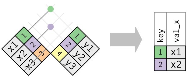
gather()：对于table4a来说，其存在两列1999/2000对应相同的变量值。故需要合并，合并后的两列重新起名字，根据key=""，和value=""。
- table4a %>% gather(1999,2000,key="year",value="cases")
- pivot_longer(c(1999,2000),names_to="year",values_to="cases")
  
  image

tidy4a <- table4a %>% 
  pivot_longer(c(`1999`, `2000`), names_to = "year", values_to = "cases")
tidy4b <- table4b %>% 
  pivot_longer(c(`1999`, `2000`), names_to = "year", values_to = "population")
left_join(tidy4a, tidy4b)
#> Joining, by = c("country", "year")
#> # A tibble: 6 x 4
#>   country     year   cases population
#>                  
#> 1 Afghanistan 1999     745   19987071
#> 2 Afghanistan 2000    2666   20595360
#> 3 Brazil      1999   37737  172006362
#> 4 Brazil      2000   80488  174504898
#> 5 China       1999  212258 1272915272
#> 6 China       2000  213766 1280428583

spread()：对于table2来说，存在冗余。需要拆分出多个变量
- table2 %>% spread(table2,key=type,value=count)
- pivot_wider(names_from = type,values_from=count)
  
  image
separate()：对于table3来说，rate一列数据可以拆分。
- separate(table3,rate,into=c("cases","population"))
  
  image
- sep=参数默认是以非数字非字母的字符为分隔符，也可以指定分隔符根据正则匹配。sep=4表示以4个字符作为分隔符。
- ==convert = TRUE表示改变分割后的数据结构。separate()默认切割后的数据结构是character。==
unite()：对指定两列合并处理。
- unite(new,centry,year,sep="")
  
  image

rename()，rename_all()： 对variables变量进行重命名。通过library(stringr)。
- rename_all(tolower) %>% rename_all(~str_replace_all(., "\\.", "_"))
mutate()，mutate_all()：对所有的value进行重命名，修改名称
- mutate_all(tolower) %>% mutate_all(~str_replace_all(., " ", "_"))
rowwise()，对每行的数据进行处理，加和/平均值处理。
- iris %>% select(contains("Length")) %>% rowwise() %>% mutate(avg_length = mean(c(Petal.Length, Sepal.Length)))

## 1 tidy_data
#### compare different dataset
table1
table2
table3
table4a;table4b

table1 %>% mutate(rate=cases/population *10000)
table1 %>% count(year,wt=cases)
ggplot(table1,aes(year,cases)) + geom_line(aes(color=country))+geom_point(color="grey")


## 2 gather()
table4a
table4a %>% gather(`1999`,`2000`,key = "year",value = "cases")
table4b %>% gather(`1999`,`2000`,key="year",value="population")
left_join(table4a,table4b,by=c("country","year"))

## 3 spread()
table2
table2 %>% spread(key = type,value = count)

stocks <- tibble(
  year=c(2015,2015,2016,2016),
  half=c(1,2,1,2),
  return=c(1.88,0.59,0.92,0.17)
)
stocks

stocks %>% spread(year,return) %>% gather("year","return",`2015`,`2016`)


## 综合操作
who %>%
  gather(new_sp_m014:newrel_f65,key="key",value="count",na.rm = T) %>%
  mutate(key=str_replace(key,"newrel","new_rel")) %>%
  separate(key,into = c("new","var","sexage"),sep="_") %>%
  select(-iso2,-iso3,-new) %>%
  separate(sexage,into = c("sex","age"),sep=1)

九，使用dplyr处理关系数据，多个数据表。

综合多个表中的数据来解决感兴趣的问题。存在于多个表中的数据称为关系数据。且关系总是定义于两个表之间的。 包括有三类操作处理关系数据：

合并数据：在一个表中添加另一个表的新变量，添加新变量的方式是以连接两个表的键来实现的。
筛选连接：在A表中，根据键是否存在于B表中来筛选这个A表中的数据。
集合操作：将观测作为集合元素来处理。

基本数据的准备包括nycflights13包中的几个表。airlines/airports/planes/weather等。

9.3 键：唯一标识观测的变量（A key is a variable (or set of variables) that uniquely identifies an observation）

主键(primary key)：唯一标识其所在数据表中的观测(不重复)例如planes$tailnum。可利用count() %>% filter(n>1)

planes %>% 
  count(tailnum) %>% 
  filter(n > 1)
#> # A tibble: 0 x 2
#> # … with 2 variables: tailnum , n 

weather %>% 
  count(year, month, day, hour, origin) %>% 
  filter(n > 1)
#> # A tibble: 3 x 6
#>    year month   day  hour origin     n
#>         
#> 1  2013    11     3     1 EWR        2
#> 2  2013    11     3     1 JFK        2
#> 3  2013    11     3     1 LGA        2

外键(foreign key)：唯一标识另一个数据表中的观测例如flights$tailnum。
代理键：当一张表没有主键，需要使用mutate()函数和row_number()函数为表加上一个主键。
理解不同数据表之间的关系的关键时：==记住每种关系只与两张表有关==，不需要清楚所有的事情，只需要明白所关心的表格即可。
- 例如 flights 与 planes相连接 via tailnum。flights 连接airlines通过carrier.等
  
  image

9.4 合并连接(mutating join)：通过两个表中的键（变量们）来匹配观测（行数值），再将一个表中的变量复制到另一个表格中。 对比cheatsheet中的信息

内连接：相当于连取交集。将两个表中的相等的键值取出来。X %>% inner_join(y,by="key")

image
外连接：至少保留存在于一个表中的观测。在另一个表中未匹配的变量会以NA表示。
- left_join() keeps all observations in x.最常用的join
- right_join() keeps all observations in y
- full_join() keeps all observations in x and y
  
  image

flights2 %>% left_join(airlines,by="carrier")
## in base R

flights2 %>% mutate(name=airlines$name[match(carrier,airlines$carrier)])

重复键：一对多（），多对一，以及多对多的关系（两表中都不唯一，会以笛卡尔积分的方式呈现）。
定义两个表中匹配的键：
- by=NULL，默认，使用存在于两个表中的所有变量。
- left_join(x,y,by="weather")
- left_join(x,y,c("dest"="faa "))
  
  image
其它Implementations: base:merge()
- Baes:merge: left_join(x, y) <=> merge(x, y, all.x = TRUE)
- SQL: left_join(x, y, by = "z") <=> SELECT * FROM x LEFT OUTER JOIN y USING (z)

9.5 筛选连接(Filtering joins)：根据键来对观测数值进行筛选，用一组数据来筛选另一组数据

semi_join(x,y,by="")：保留x表中与 y表中的观测数值相匹配的数据。
- image
anti_join(x,y)：丢弃x表中与y表中观测(行)数据相匹配的数据。
- image

9.6整理数据时需要对数据进行整理：

需要找出每个表中可以作为主键的变量。应基于数据的真实含义来找主键
确保主键中的每个变量没有缺失值，如果有缺失值则不能被识别！
检查主键是否可以与另一个表中的外键相匹配。利用anti_join()来确定。

9.7集合的操作：

intersect(x,y) 两个表中皆存在。
union()：返回x表中与y表中的唯一观测。
setdiff()：在x表中，但不在y表中的数值。

library(tidyverse)
library(nycflights13)
planes;airports;airlines;weather;


## 9.3键
weather %>% count(year,month,day,hour,origin) %>% filter(n>1) ### 筛选唯一的键

## 9.4 合并连接
flights2 <- flights %>% select(year:day,hour,origin,dest,tailnum,carrier)
flights2 %>% select(-(hour:origin)) %>% left_join(airlines,by = "carrier")
flights2 %>% select(-(hour:origin)) %>% right_join(airlines,by = "carrier")

flights2 %>% left_join(weather) ## 自然连接,使用存在于两个表中的所有变量。
flights2 %>% left_join(planes,by = "tailnum") ## 共有的
flights2 %>% left_join(airports,c("origin" = "faa"))


### exercise
##9.4.6-1目的地的平均延误时间，与空间分布。
flights %>% group_by(dest) %>% summarise(dest_delay=mean(arr_delay,na.rm = T)) %>% left_join(airports,c("dest"="faa")) %>% filter(dest_delay>0)%>%ggplot(aes(lon,lat))+borders("state")+geom_point(aes(size=dest_delay))

airports %>% semi_join(flights,c("faa"="dest")) %>% ggplot(aes(lon,lat))+borders("state")+geom_point()
##exercise3 飞机的机龄与延误时间
flights %>% group_by(tailnum) %>% summarise(count=n(),delay_tailnum=mean(arr_delay,na.rm = T)) %>% left_join(planes,by="tailnum") %>% filter(!is.na(year)) %>% ggplot(aes(x=delay_tailnum))+geom_freqpoly(aes(color=year),binwidth=1)
###geom_ribbon作图

## 9.5 筛选连接
(top_dest <- flights %>% count(dest,sort = T) %>% head(10))
flights %>% filter(dest %in% top_dest$dest)

flights %>% semi_join(top_dest,by = "dest")

十章使用stringr处理字符串。

字符串通常包含的是非结构化或者半结构化的数据。

10.1 字符串基础

R基础函数中含有一些字符串处理函数，但方法不一致，不便于记忆。推荐使用stringr函数。函数是以str_开头

字符串的长度length: str_length()
字符串的组合combine: str_c("x","y",sep = "_")
- 向量化函数，自动循环短向量，使得其与最长的向量具有相同的长度
- x <- c("abc", NA) ; str_c("1_",str_replace_na(x),"_1")
字符串character取子集subsetting strings(==根据位置==)：str_sub(x, start, end)。如果是一个向量，则对向量中的每个字符串操作，截取子集
- 对向量x<- c("Apple","Banana", "Pear")中的每个字符串第一个字母小写化。==str_sub(x,1,1) <- str_to_lower(str_sub(x,1,1))==
文本转化为大小写：全部大写str_to_upper(), 首字母大写str_to_title()
对向量内的strings按照ENGLISH进行排序：str_sort(c("apple","eggplant","banana"), locale="en")

10.2 正则匹配

利用str_view()学习正则匹配，需安装library(htmltools), htmlwidgets

str_view(x, "abc")
锚点：^ $; 单词边界：\b,如匹配一个单词 \bsum\b
特殊匹配符号：\\d, \\s, \\w, [abc], [^abc]不匹配a/b/c
数量：? + * {n,m} (..)\\1
分组和反引用：(..)\\1

10.3 各类匹配操作

匹配检测：返回逻辑值TURE(1) or FALSE(0) ==str_detect(x, "e$")==
- 利用sum(), mean()简单统计匹配的个数。
- 逻辑取子集方法筛选：words[str_detect(words,"x$")]
- 与dplyr使用的另一种技巧 ：df %>% filter(str_detect(words,"ab"))
- 等同于== str_subset(words,"x$") ==
- ==str_count(words, "[aeiou]")== 返回字符串中匹配的数量。
- 与dplyr一起使用：df %>% mutate( vowels=str_count(w,"[aeiou]"))
提取匹配的内容：== str_extract() == 只提取第一个匹配的内容。
- str_extract_all(words,color_match)返回一个列表，包含所有匹配的内容。
- str_extract_all(words,color_match, simplify= TRUE) 返回的是一个矩阵。
- 注意与str_subset()区别，subset是取子集，取所有匹配到的，无匹配的舍去。子集。而extract是取匹配到的字符串，无匹配到字符串返回NA。可先利用str_subset()找到包含匹配的chr，再用str_extract() 找到包含的匹配。
- str_match()
- 利用tidyr里的== extract() ==将字符串向量提取匹配的字符串并转变为tibble
- image
替换匹配的内容 str_replace(words, "match_x", "replace_x")
- 同时替换多个匹配的内容：str_replace_all()
- 同时执行多个替换：str_replace_all(words,c("1"="one","2"="two","3"="three"))
- image
拆分 split(sentences," ")返回的是一个列表
- "a|b|c|d" %>% str_split("\\|") %>% .[[1]]
- 内置的单词边界函数boundary()，会自动识别单词外的字符str_split(x, boundary("word"))
定位：str_locate返回匹配在字符串中的位置。
- 使用str_locate()找出匹配的模式，再用str_sub()提取或修改匹配的内容。
其它模式：
- regex()
- fixed()
- coll()

10.5 其它类型的匹配

对于一个匹配的"pattern"来说，其完整的写法是regex("pattern")。而regex()函数中包含其它的参数

ignore_case=T忽略匹配的大小写
multiline=T 可以跨行匹配
comments = T 可以添加注释信息
dotall=T可以匹配所有字符

其它应用：当想不起函数名称时可以apropos("pattern")

函数	功能说明	R Base中对应函数
使用正则表达式的函数
str_subset()	返回匹配到的子集列表
str_extract()	提取首个匹配模式的字符	regmatches()
str_extract_all()	提取所有匹配模式的字符	regmatches()
str_locate()	返回首个匹配模式的字符的位置	regexpr()
str_locate_all()	返回所有匹配模式的字符的位置	gregexpr()
str_replace()	替换首个匹配模式	sub()
str_replace_all()	替换所有匹配模式	gsub()
str_split()	按照模式分割字符串	strsplit()
str_split_fixed()	按照模式将字符串分割成指定个数	-
str_detect()	检测字符是否存在某些指定模式	grepl()
str_count()	返回指定模式出现的次数	-
其他重要函数
str_sub()	提取指定位置的字符	regmatches()
str_dup()	丢弃指定位置的字符	-
str_length()	返回字符的长度	nchar()
str_pad()	填补字符	-
str_trim()	丢弃填充，如去掉字符前后的空格	-
str_c()	连接字符	paste(),paste0()

## 10.2 字符串基础
str_length(c("a","aaaaa",NA)) ## str_length 返回字符串中的字符数量
str_c("x","y","z",sep = " ")
str_c("aaa",str_replace_na(c("bbb",NA)),"ccc")

x <- c("Apple","Banana","Pear")
(str_sub(x,1,1) <- str_to_lower(str_sub(x,1,1)))## 对首字母改为小写。
x


## 10.3正则表达式进行模式匹配。
str_view(x,".a")
str_view(x,"^a")

str_view(words,"^.{7,}$",match = T) ## exercise 只显示7个字母及以上的单词


## 10.4.1匹配检测
df <- tibble(w=words,i=seq_along(words))
df %>% filter(str_detect(w,"ab")) ##对于tibble表中筛选。
str_subset(words,"^y")

mean(str_count(words,"[aeiou]")) ## 每个单词中元音字母的数量
df %>% mutate(vowels=str_count(w,"[aeiou]"),consonants=str_count(w,"[^aeiou]")) ## 与mutate一起使用，加一列匹配到元音字母与非元音字母的数

####exercises
str_subset(words,"x$|^y")
words[str_detect(words,"x$|^y")]


## 10.4.3 提取匹配内容
colors <- c("red","orange","yellow","green","blue","purple")
(color_match <- str_c(colors,collapse = "|"))
has_color <- str_subset(sentences,color_match) ## 提取包含匹配的整个句子
matches <- str_extract(has_color,color_match) ##匹配包含匹配句子 的 第一个匹配内容。
str(matches)
###exercises
str_extract(sentences,"^\\S+")
str_extract_all(sentences,"\\w+s")

words_ing <- str_subset(sentences,"\\b\\w+ing\\b")
str_extract_all(words_ing,"\\b\\w+ing\\b")
## 10.4.5 分组匹配
noun <- "(a|the) (\\S+)"
has_noun <- sentences %>% str_subset(noun)
has_noun %>% str_extract(noun) 

sentences %>% str_subset(noun) %>% str_extract(noun)
str_match(has_noun,noun) ## 可以给出每个独立的分组，返回的是一个矩阵。
tibble(sentence=sentences) %>% extract(col = sentence,into = c("article","noun"),regex = "(a|the) (\\w+)",remove = F)

## 10.4.7 替换
str_replace()
str_replace_all(words,c("1"="one","2"="two","3"="three"))


## 10.4.9拆分
"a|b|c|d" %>% str_split("\\|") %>% .[[1]]
x <- "This is a sentence"
str_view_all(x,boundary("word"))  ## 返回句子中的所有单词

apropos("str")

十一章使用forcats处理因子

因子在R中用于处理分类变量。分类变量是在固定的已知集合中取值的变量。

使用因子时，最常用的两种操作时修改水平的顺序和水平的值。

factor(x1,levels=c("a","b","c"))
fct_reorder() ## 重新对factor的层级进行确定。
利用gss_cat数据集，其中一个问题待解决“美国民主党/共和党/中间派的人数比例是如何随时间而变化的”

relig_summary <- gss_cat %>%
  group_by(relig) %>%
  summarise(
    age = mean(age, na.rm = TRUE),
    tvhours = mean(tvhours, na.rm = TRUE),
    n = n()
  )

ggplot(relig_summary, aes(tvhours, fct_reorder(relig, tvhours))) +
  geom_point()

### 排序
relig_summary %>%
  mutate(relig = fct_reorder(relig, tvhours)) %>%
  ggplot(aes(tvhours, relig)) +
    geom_point()

十四章函数(Functions)

当一段代码需要多次使用的时候就可以写函数来实现。先编写工作代码，而后再转换成函数的代码。包括名称/参数/主体代码

range()返回最小值、最大值

library(tidyverse)
df <- tibble(a=rnorm(10),
             b=rnorm(10),
             c=rnorm(10),
             d=rnorm(10)
)
x <- df$a
rng <- range(x,na.rm = T) ## range函数返回（最大值和最小值）
(x-rng[1])/(rng[2]-rng[1])

#### 具体函数
rescale01 <- function(x){
  rng <- range(x,na.rm = T,finite=T)
  (x-rng[1])/(rng[2]-rng[1])
} ###函数名称为rescale01
rescale01(c(df$a,Inf))

#### exercises
#1, parameters
rescale01_v2 <- function(x,na.rm_TorF,finite_TorF){
  rng <- range(x,na.rm = na.rm,finite=finite)
  (x-rng[1])/(rng[2]-rng[1])
}

#2, reverse_Inf

命名的规则：函数名一般为动词，参数为名词。使用注释来解释代码。
- 一些广义的动词例如：get, compute, calculate, determine。
- 如果一组函数功能相似，可以类似于stringr包中的str_combine等改后缀的方法。
- ==Ctrl + Shift + R== 添加分节的符号

## exercises
#1,
f1 <- function(string,prefix){
  substr(string,1,nchar(prefix))==prefix
}
f3 <- function(x,y){
  rep(y,length.out(x))
}

条件执行(condition execution)：if..else..语句
- condition的值T or F
- if..else语句中使用逻辑表达式：&& ，||
- 向量化操作符： &,| 只可以用于多个值。
- 在测试相等关系时，注意 ==是向量化，容易输出多个值。
- if .. else if .. else if .. else.


## exercise2欢迎函数
greet <- function(time=lubridate::now()){
  hr <- lubridate::hour(time)
  if(hr<12){
    print("Good morning!")
  }else if (hr<18) {
    print("Good afternoon")
  }else{
    print("Good evening")
  }
}

## exercise3
fizzbuzz <- function(x){
  ###限定输入的内容格式
  stopifnot(length(x)==1)
  stopifnot(is.numeric(x))
  
  if (x%%3==0 && x%%5!=0) {
    print("fizz")
  }else if (x%%5==0 && x%%3!=0) {
    print("buzz")
  }else if (x%%5==0 && x%%3==0) {
    print("fizzbuzz")
  }else{
    print(x)
  }
}

函数的参数：主要包括进行计算的数据，控制计算过程的细节，细节参数一般都有默认值
- 检查参数值：stopifnot()
- ...捕获任意数量的未匹配的参数，将这些捕获的值传递给另一个函数。
返回值：通常是返回最后一个语句的值，可以通过return()提前返回一个值
- 检查语句是否有误。

## 使用近似正态分布计算均值两端的置信区间
mean_ci <- function(x,confidence=0.95){
  se <- sd(x)/sqrt(length(x))
  alpha <- 1-confidence
  mean(x)+se*qnorm(c(alpha/2,1-alpha/2))
}

十五章，向量vectors

一. 向量概括

向量vectors包括两种：原子向量(atomic vectors)和列表(list)

原子向量 ：包括6种：logical,numeric(integer, double), character, complex, raw。向量种的各个值都是同种类型的；
列表：递归向量，列表中也可包括其它列表。列表中的各个值可以是不同类型的。
拓展向量：向量中任意添加额外的元数据。
探索函数：typeof(), length()

image

二. 原子向量

逻辑型(logical)包括三种：TRUE, FALSE, NA
数值型(numeric):默认数值为双精度型double；
- 注意双精度型double是近似值(approximations)，所有的双精度值都当做是近似值处理，表示浮点数(floating point)
- interger的特殊数据NA,double的特殊数据NA, NaN,Inf,-Inf需要以is.finite()等判断
字符串(character)：可以包含任意数量的数据。

三. 原子向量的操作

强制转换：将一种原子强制转化为另一种；或者系统自动转化
- 显示型强制转化：as.numeric,as.character等；
- 隐式强制转化：联系上下文context自动转化，如logical(T/F)———>numeric(1/0);

x <- sample(x = 20,size = 100,replace = T)
y <- x>10
mean(y);sum(y)

检验是否为某一原子向量：利用purrr包中的函数is_ ：is_logical(), is_character等
标量与循环的规则：处理不同长度的向量会遵循 向量循环规则。例如1:10+1:3：R会拓展较短的向量，使其与较长的向量一样长。然后再相加。
向量命名：所有类型的向量都是可以命名的.向量完成后利用：purrr::set_names(x,nm=c("q","w","e"))命名。
向量的取子集：filter()函数对tibble使用，对于向量的筛选则使用[]。
- 整数型数值向量进行筛选：x[c(1,2,2,4)], x[c(-1,-2,-3)]
- ==使用逻辑向量取子集，提取出TRUE值对应的元素==。可利用比较函数
- 对命名向量可用字符取子集
- x[] 代表选取x中的全部元素，对于矩阵十分重要x[2,],x[,-3]；特殊的，[[]] 代表只提取单个元素。明确表示需要提取单个元素时使用

四. 列表（递归向量recrusive vectors）

列表是建立在原子向量基础上的一种复杂形式，列表可以包含其它列表。列表保存层级结构，树形结构。str()，重点关注列表的结构。

image

列表取子集 :
- []提取子列表，返回的是一个子列表；可用逻辑向量，整数向量，字符向量提取。
- 使用[[]]从列表中提取单个元素，并非子列表。
- 直接使用$，作用相同于[[]]。综合使用。x[[1]][[1]]
- 注意于tibble之间使用的异同点，tibble[1], tibble[[1]]

a <- list(a=1:3,b="a string",c=pi,d=list(-1,-5))
a[c(1:2)]
a["a"]
a[["a"]][1:2]

五. 特性：

任何向量都可以通过其特性来附加任意元数据。可以将特性看作可以附加在任何对象上的一个向量命名列表。维度、名称、类

泛型函数：可以根据不同类型的输入而进行不同的操作。面向对象编程的关键。可以根据不同类型的输入而进行不同的操作。例如 as.Data()

六. 拓展向量：

利用基础的原子向量和列表构建出的另外一些重要的向量类型，称为拓展向量，其具有类的附加特性。

因子：在整数型向量的基础上构建的，添加了水平特征。表示有次序的分类数据factor(c("ef","cd","ab"),levels=c("ab","cd","ef"))
日期和日期时间：数值型的向量。
tibble：拓展的列表。

Charpter16_purrr Iteration

迭代Iteration：对多个列或多个数据集进行相同的操作。两种迭代方式：

命令型编程：while(), for()。
函数式编程。减少重复代码。

一. For循环

需为输出结果分配出足够的空间。对循环效率十分重要。
涉及的函数包括 ==vector("double",ncol(df)), seq_along(df), [[]]==
1. output
2. for loop sequence
3. the body

###16.2 for循环
require(tidyverse)
df <- tibble(a=rnorm(10),
             b=rnorm(10),
             c=rnorm(10),
             d=rnorm(10))

output <- vector("double",ncol(df))
output
for (i in seq_along(df)) {
  output[i] <- median(df[[i]])
}
output


### exercise Alice the Camel
humps <- c("five", "four","three","two","one","no")
for (i in humps) {
  cat(str_c("Alice the camel has",rep(i,3),"horse",collapse = "\n"),"\n")
}

二. for循环的变体

修改现有对象：与自定义的函数function()一起使用。
- 注意在循环loop中，所有for循环使用的都是[[]] ，明确表示是要处理单个元素。
- df[[i]] = rescale01(df[[i]])

### create a tibble
df <- tibble(
  a = rnorm(10),
  b = rnorm(10),
  c = rnorm(10),
  d = rnorm(10)
)

### create a function
rescale01 <- function(x) {
  rng <- range(x, na.rm = TRUE)
  (x - rng[1]) / (rng[2] - rng[1])
}

### use the loop
for (i in )

循环模式：
- 通过对数值索引进行循环，再通过x[[i]]提取相应的值。
- 通过对元素element索引。
- 通过使用名称索引：for (i in names(x))，需要使用元素的名称时使用。有利于图表标题和文件名
处理未知的输出长度。
- 应该将loop每次的结果保存再一个列表中，循环结束后再利用unlist() 或者purrr::flatten_dbl()组合成一个向量
- 当遇到类似的问题，如生成一个很长的字符串paste(out,collapse="")，或是个很大的数据框 ==rbind_rows(), unlist()== 。应首先使用一个更复杂的对象来保存每次迭代的结果，最后再一次性的组合起来。

means <- c(0,1,2)
output <- double()
for (i in seq_along(means)) {
  n <- sample(100,1)
  output <- c(output,rnorm(n,mean = means[[i]])) ### 十分不高效，这里会复制上一次的所有数据。
}

##高效法 
out <- vector("list",length = length(means))
for (i in seq_along(means)){
  n <- sample(100,1)
  out[[i]] <- rnorm(n,mean = means[[i]])
}
unlist(out)

处理未知长度的序列。利用while循环来实现。

for (i in seq_along(x)){
    # body
}

## equivalent to 
i <- 1
while(i <= length(x)){
    # body
    i<- i + 1
}

Exercises

####exercises
# 1.读取文件，保存在大的数据框中
files <- dir(path = ".",pattern = "tsv$",full.names = F) ###匹配某一路径下所有的文件。
data_list <- vector("list",length = length(files))
for (i in seq_along(files)) {
  data_list[[i]] <- read_delim(files[[i]],delim = "\t")
}
bind_rows(data_list)

#2.输出所有df中数值列的均值及名称show_mean(iris)
iris <- as_tibble(iris)
show_means <- function(df,digits=2){
  maxstr <- max(str_length(names(df)))
  for (i in names(df)) {
  if (is.numeric(df[[i]])) {
    cat(
      str_c(str_pad(str_c(i,":"),maxstr+1L,side = "right"),
            format(mean(df[[i]]),digits=2,nsmall=2),
                   sep=" "
              ),
     sep =  "\n"  
    )
  }
}
}

三. for循环与函数式编程

函数式编程语言意味着可以先将for循环包装在函数中。即将函数名作为参数传入到另一个函数中
利用purrr函数，可以将复杂问题解决成子问题，然后再通过管道操作将这些问题的结果组合起来。

col_summary <- function(x,fun){
  out <- vector("double",length(x))
  for (i in seq_along(x)) {
    out[[i]]=fun(x[[i]])
  }
  out
}

## so, we can use a funtion in fun parameter.

col_summary(df,median) ## calculate the median value of each column.

四. 映射函数 The map function.

purrr包函数map()(返回的是列表),map_lgl(),map_dbl(),map_chr()。map()第二个参数可以是公式，字符向量，整型向量，==...== 作为.function 的附加参数。第三个参数为第二个函数中的附加参数。例如： map_dbl(df, mean, trim = 0.5)。在对列表中的各个子集内部进行筛选，返回的依旧是个列表

快捷方式(shortcuts)：对某个数据集中的每个分组都拟合一个线性模型。类似于factor中的一些功能。
- ==.== 作为一个代词，代表当前的列表元素。
- ==~== 作为function(x)
- ==~.$r.squared== 结合
- 提取命名成分map_dbl(~.$r.squared), or map_dbl(2)循环取列表里的第2个值。
BaseR 中的apply函数组。lapply(), sapply(), vapply()。而purrr作为Hardley开发的，具有更加一致的map_*名字和参数，. ~的快捷方式，并行计算，以及计算的进度条。
exercises中涉及的一些函数：map(-2:2,rnorm, n=5), map(1:3,rnorm,mean=10).
对操作失败的处理：safely(), possibly(), quietly()

### split 分割出列表
models <- mtcars %>% 
  split(.$cyl) %>% 
  map(function(df) lm(mpg ~ wt,data=df)) ##  df是一个匿名函数，可任意命名。
  
## alias:
models <- mtcars %>% split( .$cyl) %>% map( ~ lm(mpg ~ wt,data=.))

### extract the componet
models %>% 
  map(summary) %>% 
  map_dbl(~.$r.squared)
#>     4     6     8 
#> 0.509 0.465 0.423

map(out, ~ .[. > 0.8]) ###筛选每一列中大于0.8的数据。

map(df,function(xxx) length(unique(xxx))`——》`map(df, ~ length(unique(.)))

五. 多参数映射mapping over multiple arguments

map2(), pmap()对每一列的功能操作会涉及到多个参数时，就需要利用此函数。注意每次调用时候，发生变化的参数放在函数功能的前面位置，值保持不变的参数放在映射函数的后面；参数为list

mu <- list(5,10,-3)
map(mu, rnorm, n=5)
### map2 的应用
sigma <- list(1,5,10)
map2(mu,sigma,rnorm,n=5)
### pmap()应用，多个参数都未定，就将参数保存到大列表中
n <- list(3,5,8)
args <- list(n=n,sd=sigma,mean=mu)
pmap(args,rnorm)

image

多个参数 对于pmap()函数，可以将多个输入列表作为参数。且多个列表的长度一样**可以转换为tibble，确保每列都有名称，且与其它列具有相同的长度 **

image

params <- tribble(
  ~mean, ~sd, ~n,
    5,     1,  1,
   10,     5,  3,
   -3,    10,  5
)
params %>% 
  pmap(rnorm)
#> [[1]]
#> [1] 6.02
#> 
#> [[2]]
#> [1]  8.68 18.29  6.13
#> 
#> [[3]]
#> [1] -12.24  -5.76  -8.93  -4.22   8.80

多个参数，且多个映射函数，利用invoke_map()函数，参数不同，甚至函数本身也不同。（invoke 调用）

六. 游走函数，预测函数，归纳与累计

游走函数walk，输出保存多个文件时非常实用。walk(), pwalk()。
- 例如有一个图形列表和一个文件名的向量，可以使用pwalk()将每个文件保存到相应的位置。

library(ggplot2)
plots <- mtcars %>% split(.$cyl) %>% 
  map( ~ ggplot(data = .,mapping = aes(mpg,wt))+geom_point())
  path=stringi::stri_c(names(plots),".pdf")
  
  pwalk(list(path,plots),ggsave,path=tempdir())

预测函数keep(), discard()函数可以保留输入中预测值为TRUE和FALSE的元素。some(), every()分别用来确定预测值是否对某个元素为真。detect()找出预测值为真的第一个元素，detect_index()返回找到的元素的位置。
归纳约简与累计 reduce/accumulate：复杂列表简化为一个简单列表。

vs <- list(c(1,2,3,4,5),
           c(1,2,3,4),
           c(1,2,3))
reduce(vs,intersect)

charpter21_ggplot2(graphics for communication)

标签labels:labs()
- title="" 主标题
- subtitle="" 副标题，添加附加信息；
- caption= " " 描述数据来源 右下角添加信息
- x=" ", y=" "坐标轴信息
- color= "" 图例中的标题
- x= quote() 坐标轴上使用数学公式

library(ggplot2)
require(tidyverse)
ggplot(mpg,aes(displ,hwy))+geom_point(aes(color=class))+labs(title = "aaaaa",subtitle = "bbbbb",caption = "cccc ",x="HWY",y="DISPL")

注释Annotation：为单个或分组的观测值添加标签。
- filter(row_number(desc(hwy))==1) 筛选每个组中hwy数值最高的观测observation。
- geom_point() + geom_text(aes(label= ),data=)
- 利用ggrepel包可以自动调整注释标签的位置 geom_label_repel(aes(label=))
- 将标题加在图形里的右上角角落上
- 添加参考线geom_hline(),geom_vline(size=2,color=white)
- 感兴趣的点周围添加个矩形 geom_rect()
- 绘制箭头，指向关注的数据点geom_segment()

library(ggplot2)
library(ggrepel)
best_in_class <- mpg %>% group_by(class) %>% filter(row_number(desc(hwy))==1)
ggplot(mpg,aes(displ,hwy))+geom_point(aes(color=class))+geom_text(mapping = aes(label=model),data = best_in_class)
### 利用ggrepel用较大的空心圆来强调
ggplot(mpg,aes(displ,hwy))+geom_point(aes(color=class))+geom_point(size=4,shape=1,data = best_in_class)+geom_label_repel(aes(label=model),data = best_in_class)

### 将标题加在图形里的右上角角落上。
label <- mpg %>% summarise(displ=max(displ),hwy=max(hwy),label="AAAA\nbbbbbbbb")
ggplot(mpg,aes(displ,hwy))+geom_point()+geom_text(aes(label=label),data = label,vjust="top",hjust="right")

标度scale:控制从数据值到图形属性的映射。scale_x（图形属性名称）_continuous()（连续型/离散型/时间/日期时间型）
- 调整坐标轴axis ticks： 刻度 scale_y_continuous(breaks=seq(1,40,by=5)),坐标轴图例项目scale_y_continuous(labels=NULL)
- 图例legend:theme(legend.position="none/right/left/top/bottom"), 控制图例的显示guides(guide_legend())
- 标度替换：对标度进行数学转换。
- 颜色的转换：利用RColorBrewer/ggsci包,对于数量少的legend，可以添加形状映射。

ggplot(mpg,aes(displ,hwy))+geom_point(aes(color=class))+geom_smooth(se=F,color="darkgrey")+theme(legend.position = "bottom")+guides(color=guide_legend(nrow = 1,override.aes = list(size=4)))

library(ggsci)
library(RColorBrewer)
ggplot(mpg,aes(displ,hwy))+geom_point(aes(color=drv))+scale_color_brewer(palette = "Set1")
ggplot(mpg,aes(displ,hwy))+geom_point(aes(color=drv,shape=drv))+scale_color_aaas()

缩放，控制图形范围。coord_cartesian()函数设置xlim和ylim的参数值。
主题(themes)：定制图形中的非数据元素。theme_bw(),theme_grey()（默认）,theme_classic(),theme_light()
保存图形ggsave()

R数据科学 R for data sciences

前言

一 使用ggplot2进行数据可视化

二 工作流：基础 Workflow：basics

三 使用dplyr进行数据转换

五，探索性数据分析 exploratory data analysis(EDA)

七， tibble

八， 使用readr进行数据的导入

九，使用tidyr整理数据表 Tidy data

九，使用dplyr处理关系数据，多个数据表。

十章 使用stringr处理字符串。

10.1 字符串基础

10.2 正则匹配

10.3 各类匹配操作

10.5 其它类型的匹配

十一章 使用forcats处理因子

十四章 函数(Functions)

十五章， 向量vectors

一. 向量概括

二. 原子向量

三. 原子向量的操作

四. 列表（递归向量recrusive vectors）

五. 特性：

六. 拓展向量：

Charpter16_purrr Iteration

一. For循环

二. for循环的变体

三. for循环与函数式编程

四. 映射函数 The map function.

五. 多参数映射mapping over multiple arguments

六. 游走函数，预测函数，归纳与累计

charpter21_ggplot2(graphics for communication)

你可能感兴趣的:(R数据科学 R for data sciences)

一使用ggplot2进行数据可视化

二工作流：基础 Workflow：basics

三使用dplyr进行数据转换

八，使用readr进行数据的导入

十章使用stringr处理字符串。

十一章使用forcats处理因子

十四章函数(Functions)

十五章，向量vectors