2019.5.18
人生苦短,我用Python。最近关于Python的学习是真的多,我也只能多线程地来学习了。今天丁烨老师上传了最新的教案pdf,所以从今天开始,我又往我近期的列表里append了Pandas的学习。

一.Pandas模块
1. 概述
Pandas官网
pandas 是一个开源的,BSD许可的库,为Python编程语言提供高性能,易于使用的数据结构和数据分析工具。Python长期以来一直非常适合数据整理和准备,但对于数据分析和建模则不那么重要。pandas有助于填补这一空白,使您能够在Python中执行整个数据分析工作流程,而无需切换到更像域的特定语言,如R语言。
简而言之,pandas是超越了numpy的一个数据处理和数据建模的模块。 它具备了对数据的预处理,生成单列数据,以及比numpy更为强大的数据结构,并且可以做出类似于SQL数据库的操作,并可以直接使用numpy的值,更可以将数据导出成csv、Excel表等强大功能。
2.用法
- 两种建模方式
- Series:一维的、可带标签的同构数组对象(类似于数据库中的一个字段,即一列)
- DataFrame: 二维的、可带标签的同构数组。每一列必须同构,不同列可以异构。(类似于数据库中的一个关系表)
- tips:Pandas不适合处理高维的数据。
-
创建对象
Series可以通过列表或者元组来初始化,DataFrame可以通过一个Numpy数组或者字典来初始化。下面使用到的pandas.date_range()是用于生成日期范围的函数,在这个例子中,用于生成作为索引的日期。
import numpy as np
import pandas as pd
# 直接利用一个列表来初始化Series,其中numpy.nan是类似于NULL的存在
s = pd.Series([1, 3, 5, np.nan, 6, 8])
print(s)
"""Output
0    1.0
1    3.0
2    5.0
3    NaN # 输出空值
4    6.0
5    8.0
dtype: float64 #数值默认为float型
"""
dates = pd.date_range('20130101', periods=6) # 生成日期范围的函数,起始日期为2013/01/01,时期为6天
print(dates)
"""Output
DatetimeIndex(['2013-01-01', '2013-01-02', '2013-01-03', '2013-01-04',
            '2013-01-05', '2013-01-06'],
           dtype='datetime64[ns]', freq='D')
"""
# 通过Numpy数组来生成DataFrame对象,并以上面生成的日期范围作为索引,属性列也命名为'ABCD'这四个值。
df = pd.DataFrame(np.random.randn(6, 4), index=dates, columns=list('ABCD'))
print(df)
"""Output
               A          B         C         D
2013-01-01 -1.970029  2.080632 -0.450484 -0.149300
2013-01-02  0.202809 -2.384539 -0.295012 -0.419630
2013-01-03  0.436642 -0.214195 -1.677464  0.545785
2013-01-04  0.809162 -0.489416  0.379824  1.168125
2013-01-05 -0.846945  1.277425 -1.383941 -1.921999
2013-01-06 -0.174712 -0.063350 -0.265923 -0.233885
"""
# 你还可以用通过一个字典来初始化DataFrame对象,Timestamp是一个时间戳函数
df2 = pd.DataFrame({'A': 1., 'B': pd.Timestamp('20130102'), 'C': pd.Series(1, index=list(range(4)), dtype='float32'), 'D': np.array([3] * 4, dtype='int32'), 'E': pd.Categorical(["test", "train", "test", "train"]), 'F': 'foo'})
print(df2) # 可以看到,字典的键成为了列的属性名。
"""Output
    A      B        C   D     E    F
0  1.0 2013-01-02  1.0  3   test  foo
1  1.0 2013-01-02  1.0  3  train  foo
2  1.0 2013-01-02  1.0  3   test  foo
3  1.0 2013-01-02  1.0  3  train  foo
"""
print(df2.dtypes) # DataFrame很像关系型数据库的一张关系表,每一列可以异构,但同一列必须同构
"""Output
A           float64
B    datetime64[ns]
C           float32
D             int32
E          category
F            object
dtype: object
"""
-
数据的访问
DataFrame对象中许多的方法可以对其中的特定数据进行访问。例如head()、tail()等,其中又有很多属性可以访问特定的值。以下会举一些常用的例子。DataFrame提供了一个可以让自己转换为Numpy数据的函数to_numpy()* ,但Pandas 和 NumPy 有结构上的本质区别*: Pandas 允许 DataFrame 中的每一列数据设置为不同的数据结构;而 NumPy 要求整个数组同构。 当使用 DataFrame.to_numpy() 时,Pandas 将寻找 NumPy 中最近的能表达原始数据dtype。如果 dtype 不同,Pandas 将对每一个数据元素调用格式转换函数。 因此,当 DataFrame 元素较多的时候,此函数将消耗大量时间
print(df.head()) # 输出DataFrame对象的开头几行。默认是前5行,可以自定义
"""Output
                A         B         C         D
2013-01-01 -1.970029  2.080632 -0.450484 -0.149300
2013-01-02  0.202809 -2.384539 -0.295012 -0.419630
2013-01-03  0.436642 -0.214195 -1.677464  0.545785
2013-01-04  0.809162 -0.489416  0.379824  1.168125
2013-01-05 -0.846945  1.277425 -1.383941 -1.921999
"""
print(df.tail(2)) # 输出DataFrame对象的末尾几行。与head()一样输出的行数可以自定义,这里自定义为输出最后两行
"""Output
                A         B         C         D
2013-01-05 -0.846945  1.277425 -1.383941 -1.921999
2013-01-06 -0.174712 -0.063350 -0.265923 -0.233885
"""
print(df.index) # 输出索引值
"""Output
DatetimeIndex(['2013-01-01', '2013-01-02', '2013-01-03', '2013-01-04',
            '2013-01-05', '2013-01-06'],
           dtype='datetime64[ns]', freq='D')
"""
print(df.columns) # 输出列属性名
"""Output
Index(['A', 'B', 'C', 'D'], dtype='object')
"""
print(df.to_numpy()) # 将DataFrame转换为Numpy数组
"""Output
[[-1.97002931  2.08063244 -0.45048393 -0.14929988]
 [ 0.20280913 -2.38453931 -0.29501209 -0.41962973]
 [ 0.43664217 -0.21419501 -1.67746363  0.54578509]
 [ 0.80916191 -0.48941566  0.37982384  1.1681251 ]
 [-0.84694546  1.27742454 -1.38394127 -1.92199883]
 [-0.17471197 -0.06335029 -0.2659226  -0.23388499]]
"""
print(df2.to_numpy()) # 由于DataFrame的每一列可能不同构,所以比较复杂时,转化为Numpy数组花的时间要长一些
"""Output
[[1.0 Timestamp('2013-01-02 00:00:00') 1.0 3 'test' 'foo']
 [1.0 Timestamp('2013-01-02 00:00:00') 1.0 3 'train' 'foo']
 [1.0 Timestamp('2013-01-02 00:00:00') 1.0 3 'test' 'foo']
 [1.0 Timestamp('2013-01-02 00:00:00') 1.0 3 'train' 'foo']]
"""
print(df.describe()) # 使用 describe() 函数可以把数据的统计信息展示出来
"""Output
           A         B         C         D
count  6.000000  6.000000  6.000000  6.000000
mean  -0.257179  0.034426 -0.615500 -0.168484
std    1.011785  1.544615  0.769556  1.042999
min   -1.970029 -2.384539 -1.677464 -1.921999
25%   -0.678887 -0.420610 -1.150577 -0.373194
50%    0.014049 -0.138773 -0.372748 -0.191592
75%    0.378184  0.942231 -0.273195  0.372014
max    0.809162  2.080632  0.379824  1.168125
"""
print(df.T) # 输出DataFrame的转置矩阵
"""Output
   2013-01-01  2013-01-02  2013-01-03  2013-01-04  2013-01-05  2013-01-06
A   -1.970029    0.202809    0.436642    0.809162   -0.846945   -0.174712
B    2.080632   -2.384539   -0.214195   -0.489416    1.277425   -0.063350
C   -0.450484   -0.295012   -1.677464    0.379824   -1.383941   -0.265923
D   -0.149300   -0.419630    0.545785    1.168125   -1.921999   -0.233885
"""Output
print(df.sort_index(axis=1, ascending=False))
# 根据索引进行排序,axis表示你要排序的轴,axis=0表示竖轴,axis=1表示横轴
# 而ascending表示是否按照升序来排序,默认是True
"""Output
                D         C         B         A
2013-01-01 -0.149300 -0.450484  2.080632 -1.970029
2013-01-02 -0.419630 -0.295012 -2.384539  0.202809
2013-01-03  0.545785 -1.677464 -0.214195  0.436642
2013-01-04  1.168125  0.379824 -0.489416  0.809162
2013-01-05 -1.921999 -1.383941  1.277425 -0.846945
2013-01-06 -0.233885 -0.265923 -0.063350 -0.174712
"""
print(df.sort_values(by='B')) # 根据给定的列名,根据值的大小来排序,同样有ascending采纳数
"""Output
                A         B         C         D
2013-01-02  0.202809 -2.384539 -0.295012 -0.419630
2013-01-04  0.809162 -0.489416  0.379824  1.168125
2013-01-03  0.436642 -0.214195 -1.677464  0.545785
2013-01-06 -0.174712 -0.063350 -0.265923 -0.233885
2013-01-05 -0.846945  1.277425 -1.383941 -1.921999
2013-01-01 -1.970029  2.080632 -0.450484 -0.149300
"""
-
选取数据、索引
类似 NumPy,Pandas 亦提供了多种多样的选择数据的函数和成员变量。
# 选择一列中的数据:
print(df['A']) # 单独输出属性名为'A'的一列数据,返回一个Series对象
"""Output
2013-01-01   -2.330696
2013-01-02   -0.318615
2013-01-03    0.667367
2013-01-04    0.241847
2013-01-05    1.304542
2013-01-06   -0.343536
Freq: D, Name: A, dtype: float64
"""
# Pandas还可以通过[]来截取一部分数据,用于输出指定范围的行
print(df[0:3])
"""Output
                A         B         C         D
2013-01-01 -2.330696 -1.421068 -1.734107  2.486537
2013-01-02 -0.318615 -1.274842  0.030403 -0.133000
2013-01-03  0.667367  1.288029 -0.291147 -1.978817
"""

# 使用loc和iloc来访问数据
# loc是使用特定的标签来访问数据的
# iloc可以通过数字来定位哪行哪列的数据
print(df.loc[:, ['A', 'B']]) # pandas.DataFrame.loc可以通过标签来访问特定数据
"""Output
                A         B
2013-01-01 -2.330696 -1.421068
2013-01-02 -0.318615 -1.274842
2013-01-03  0.667367  1.288029
2013-01-04  0.241847  0.116068
2013-01-05  1.304542  0.757466
2013-01-06 -0.343536  0.542275
"""
print(df.iloc[3:5, 0:2]) # pandas.DataFrame.iloc是通过整数来访问特定数据的
"""Output
                A         B
2013-01-04  0.241847  0.116068
2013-01-05  1.304542  0.757466
"""

# 使用布尔值来选取数据
print(df[df.A > 0]) # 会输出复合条件的记录
"""Output
                A         B         C         D
2013-01-03  0.667367  1.288029 -0.291147 -1.978817
2013-01-04  0.241847  0.116068 -1.386416  1.203264
2013-01-05  1.304542  0.757466 -0.036668  1.030613
"""
-
处理缺失值
类似于Numpy和关系型数据库,数据中难免有一些空白值,而 在Pandas中,空值将会被赋值成Numpy的nan类型。 我们使用reindex函数可以方便的新增、修改、删除索引。
# 存储为空值
df1 = df.reindex(index=dates[0:4], columns=list(df.columns) + ['E']) # 为df增加一个E列,并存储在df1
df1.loc[dates[0]:dates[1], 'E'] = 1 # 只给部分数据赋值
print(df1) # 未赋值的值是NaN
"""Output
                A         B         C         D    E
2013-01-01 -2.330696 -1.421068 -1.734107  2.486537  1.0
2013-01-02 -0.318615 -1.274842  0.030403 -0.133000  1.0
2013-01-03  0.667367  1.288029 -0.291147 -1.978817  NaN
2013-01-04  0.241847  0.116068 -1.386416  1.203264  NaN
"""

# 丢弃所有空值
print(df1.dropna(how='any')) # how指定了丢弃空值的方式,这里指所有
"""Output
                A         B         C         D    E
2013-01-01 -2.330696 -1.421068 -1.734107  2.486537  1.0
2013-01-02 -0.318615 -1.274842  0.030403 -0.133000  1.0
"""

# 利用指定值填补所有的空值
print(df1.fillna(value=5)) # values为指定的值
"""Output
                A         B         C         D    E
2013-01-01 -2.330696 -1.421068 -1.734107  2.486537  1.0
2013-01-02 -0.318615 -1.274842  0.030403 -0.133000  1.0
2013-01-03  0.667367  1.288029 -0.291147 -1.978817  5.0 # NaN已经被替代为5
2013-01-04  0.241847  0.116068 -1.386416  1.203264  5.0
"""
-
像数据库一样使用DataFrame
DataFrame对象与关系型数据库的关系表相似不仅仅是因为它们都是二维表,而是DataFrame可以进行和数据库一样的数据操作。例如:自然连接、笛卡尔积等。
# 等值连接
left = pd.DataFrame({'key': ['foo', 'bar'], 'lval': [1, 2]}) # 创建两个待连接的表
right = pd.DataFrame({'key': ['foo', 'bar'], 'rval': [4, 5]})
print(pd.merge(left, right, on='key')) # on指定根据什么值相等去连接
"""Output
   key   lval   rval
0  foo     1     4
1  bar     2     5
"""
# 笛卡尔积,同样是连接,但由于有相同的键,所以会进行笛卡尔积
left = pd.DataFrame({'key': ['foo', 'foo'], 'lval': [1, 2]})
right = pd.DataFrame({'key': ['foo', 'foo'], 'rval': [4, 5]})
print(pd.merge(left, right, on='key'))
"""Output
   key   lval   rval
0  foo     1     4
1  foo     1     5
2  foo     2     4
3  foo     2     5
"""
# 分组
# 1. 将数据根据特定的条件分为几个不同的组
# 2. 对每组数据做数学操作(例如 count:清点数量)
# 3. 将结果输出成一个完整的数据结构
df = pd.DataFrame({'A': ['foo', 'bar', 'foo', 'bar', 'foo', 'bar', 'foo', 'foo'],'B': ['one', 'one', 'two', 'three', 'two', 'two', 'one', 'three'], 'C': np.random.randn(8), 'D': np.random.randn(8)})
print(df.groupby('A').sum())
"""Output
        C         D
A
bar  1.63216 -0.493714
foo  1.89041 -0.111024
"""
- 导入导出数据
Pandas除了可以自己构造数据之外,同时具有 从csv、hdf、Excel表等文件读入数据,以及将数据写到这些文件中的功能。需要注意到的是,所有的read方法都是来自于Pandas的,而所有的to(写数据到文件中)方法都是属于DataFrame的。
- 读数据:
- Pandas.read_csv()
- Pandas.read_hdf()
- Pandas.read_excel()
- 这三个函数就是Pandas分别用于从csv、hdf、Excel表三种数据文件中读取表格数据,并将其存储于一个DataFrame对象的函数(点击可跳到API文档)。
- 写数据
- Pandas.DataFrame.to_csv()
- Pandas.DataFrame.to_hdf()
- Pandas.DataFrame.to_excel()
- 这三个函数可以将DataFrame对象的数据写入到三种文件类型中去。(点击可跳到API文档)。
- 重点:
1. 使用to_excel()将数据写到excel之前需要pip安装openpyxl库。
2. to_系列的函数中,有mode, index两个参数,前者表示写数据的模式,有w、r、a(write、read、append)等,与C语言的文件读写模式相似;index则表示写数据要不要把索引写进去,默认是True,但我使用时一般设为False。
- Pandas与SQL数据库合作
Pandas除了可以自己初始化或者从文件中读取数据之外,还可以直接和数据库进行交互,运行SQL语句,读写和查询数据库的数据。
1. pymssql的安装
因为我个人使用的数据库是SQL Server,所以为了让pandas进行对mssql的操作,就要安装pymssql库,来进行mssql的操作。如果使用其他的数据库,就需要安装其他的py库。
python pip install pymssql
2. pymssql的使用练习
> * 连接到mssql数据库
> * pymssql.connect(),用于设置连接数据库的信息, server需要提供IP或者localhost,user是指用户名(默认是sa),database指需要连接的数据库的名字.返回一个connection类对象
```python
import pymssql
conn = pymssql.connect(server="127.0.0.1",user="zackary",password="*****XTZBw*****",database="master")
```
> * **读写数据库数据**
> * **pandas.read_sql** **(** **sql**, **con**, *index_col=None, coerce_float=True, params=None, parse_dates=None, columns=None, chunksize=None* **)**
**其中sql表示sql查询语句或者表名, con为connection类的对象; 返回一个DataFrame类对象,所以要用pandas库来操作**
> * **pandas.DataFrame.to_sql** **(** *name, con, schema=None, if_exists='fail', index=True, index_label=None, chunksize=None, dtype=None, method=None* **)**
> *这个是DataFrame中的写数据库的函数*,**由于read_sql( )返回的是DataFrame类的对象,所以用pandas进行相应的操作之后,可以用to_sql( )函数来将数据写入数据库,其中name是表名.** *由于不想改变我的sql表的数据,就不演示了。*
> * **由于每个人的数据库不一样,所以以下的例子需要修改成你电脑上的样子**
```python
import pandas as pd
# sql是你要执行的查询语句
sql = "select * from [master].[dbo].[MSreplication options]"
df1 = pd.read_sql(sql,conn)
print(df1)
```

二.利用pandas进行数据清理实例
练习的来源是我的《Python数据分析》的任课老师丁烨的pdf,如果你有兴趣,请点击此处。
- 读取数据
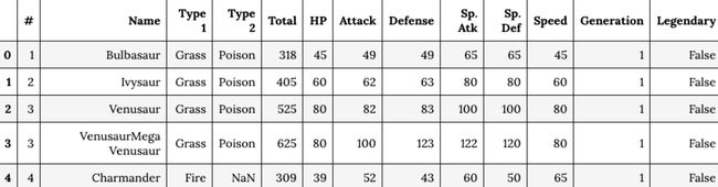
- 利用 read_csv( ) 方法将一个csv文件读入到DataFrame对象中,利用head( )查看头5行数据(实际有700多行)。
- 数据预处理
- Pandas.DataFrame.rename(mapper=None, index=None, columns=None, axis=None, copy=True, inplace=False, level=None)
可以 对参数列表内的属性进行重命名,修改方法是采用字典的方式.本例就是将名为"#"的列改名为"id",inplace参数表明要不要修改,还是临时显示修改的副本- 利用 str.lower( ) 将所有列属性的名字都改成小写
- Pandas.DataFrame.duplicated(subset=None, keep='first')
用于标记重复数据的函数,subset表示"参考为重复因素的列",等于None时表示全部列(默认);keep指不标记的那个"例外",keep有三个取值,分别是'first', 'last', False,分别表示不标记第一个,不标记最后一个,标记全部(默认)
df.rename(columns={'#': 'id'}, inplace=True)
df.columns = df.columns.str.lower()
df[df.duplicated('id', keep=False)].head()
- 清洗数据,去除重复项
- DataFrame.drop_duplicates(subset=None, keep='first', inplace=False)
用于删除重复项,这里可以看到.subset的值为'id',可知是只查找'id'列中重复的值; keep的取值为'first',指只留下重复项的第一个;inplace代表替代原数据。- df['type 2']指属性为type 2的所有数据(那一列), fillna( )会用values(这里是用了None)填补原先为numpy.na(空)的数据,这里使所有的空数据项变成None。
df.drop_duplicates('id', keep='first', inplace=True)
df['type 2'].fillna(value='None', inplace=True)
- 按需拆分表格
- pokedex拆分出df中的几个属性出来,成为了一张新表,存储id, name等信息。
- 用pandas.merge( )将df表和pokedex表进行外表连接(数据库的操作), on表示它们是在'id'相同处拼接的.同时,将id, hp, attack等属性(以及数据)赋值给statistics表,得到数据。
pokedex = df[['id', 'name', 'type 1', 'type 2', 'generation', 'legendary']]
statistics = pd.merge(df, pokedex, on='id').loc[:, ['id', 'hp', 'attack', 'defense', 'sp. atk', 'sp. def', 'speed', 'total']]
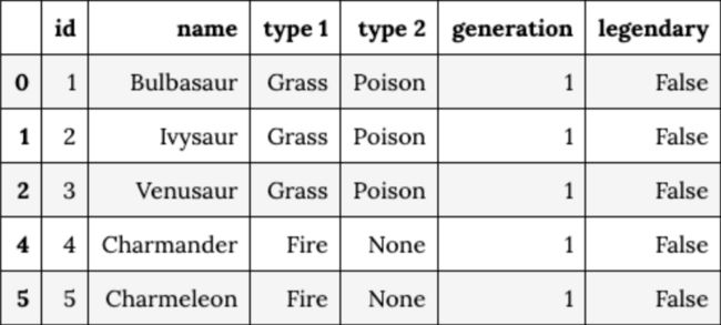 pokedex
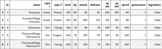
 statistics
- 使用seaborn画图
- seaborn,是一个数据可视化的库,类似于 matplotlib。
- 在linux下安装seaborn时,可能会出现这样的错误
这时候需要安装一些东西。 Error
Errorsudo apt-get install at-spi2-core
-
绘图
- seaborn可以像matplotlib一样绘图,但显示不是用seaborn,而是用pyplot.所以在使用的时候要加上plt.show()
- 丁烨老师这里的pdf是有错误的,用了中文的引号。由此我见识到了一个有趣的错误
SynataxError: EOL while scanning string literal : 当字符串的最后一个字符是斜杠或者不是ASCII码时,报错。 Error
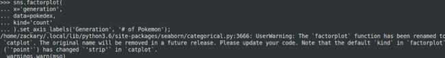
Error - factplot( )函数已改名为catplot( )
 函数名变更
函数名变更
from matplotlib import pyplot as plt sns.factorplot(x='generation', data=pokedex, kind='count').set_axis_labels('Generation', '# of Pokemon') plt.show()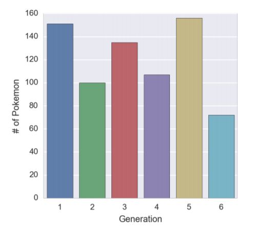 seaborn绘图
-
绘图实例
- seaborn.catplot()
catplot()拥有着十分多的参数,这里会讲解例子中用到的参数。 y代表y轴是什么,data表示数据源。通过kind生成不同类别的图, kind的取值有: strip, swarm, box, violin,boxen,point, bar, count,strip为默认值;order指排序。
sns.factorplot(y='type 1',data=pokedex,kind='count',order=pokedex['type 1'].value_counts().index,aspect=1.5,color='green').set_axis_labels('# of Pokemon', 'Type 1') sns.factorplot(y='type 2',data=pokedex,kind='count',order=pokedex['type 2'].value_counts().index,aspect=1.5,color='purple').set_axis_labels('# of Pokemon', 'Type 2')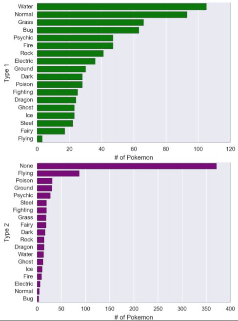 案例
案例 - seaborn.catplot()
- 统计出前十最强的宝可梦
思路:
1. 将数据的处理编写成函数便于管理
2. 用merge( )将两个表连接
3. 使用sort_values( )对table表进行排序
4. 使用catplot( )画图
import numpy as np
import pandas as pd
from matplotlib import pyplot as plt
import seaborn as sns

def dataProcess():
    """ The function is to get, select and clean the data"""
    # To get the csv file
    df = pd.read_csv('https://dingye.me/src/pokemon-v0.5.27.csv')
    df.rename(columns={'#': 'id'}, inplace=True)
    df.columns = df.columns.str.lower()
    # Just show the first five tuple
    df[df.duplicated('id', keep=False)].head()

    df.drop_duplicates('id', keep='first', inplace=True)
    df['type 2'].fillna(value='None', inplace=True)
    pokedex = df[['id', 'name', 'type 1', 'type 2', 'generation', 'legendary']]
    statistics = pd.merge(df, pokedex, on='id')
    statistics = statistics.loc[:, ['id', 'hp', 'attack', 'defense', 'sp. atk', 'sp. def', 'speed', 'total']]
    return statistics, pokedex
    """
    return pokedex
    """

if __name__ == "__main__":
    """
    pokedex = dataProcess()
    sns.catplot(x='generation', data=pokedex, kind='count').set_axis_labels('Generation', '# of Pokemon')
    # You need to use this function to show the pictures
    plt.show()
    """

    # To get, select and clean the data
    statistics, pokedex = dataProcess()
    table = pd.merge(pokedex,statistics, on='id')
    # print(table)
    table = table.sort_values(by='total', ascending=False)
    print(table)

    # Make it virtualization
    sns.catplot(x='total', y='name', data=table[:10], kind='bar').set_axis_labels('# of Top ten Pokemon', 'The total counts')
    plt.title('Top ten pokemon')
    plt.show()
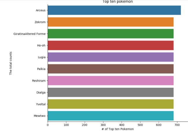 前十的宝可梦