3月29日 天气晴 心情雷暴
Preprosessing the data
import numpy as np
import pandas as pd
import matplotlib.pyplot as pl
from matplotlib import rcParams
import scanpy as sc

sc.settings.verbosity = 3  # verbosity: errors (0), warnings (1), info (2), hints (3)
sc.logging.print_versions()
scanpy==1.4 anndata==0.6.19 numpy==1.14.5 scipy==1.1.0 pandas==0.23.4 scikit-learn==0.19.2 statsmodels==0.9.0 python-igraph==0.7.1 louvain==0.6.1
adata = sc.read_h5ad("/bone_marrow/scanpy/3_29_PC16_filterMore/umap_tsne_3_29.h5ad")
sc.tl.draw_graph(adata)
drawing single-cell graph using layout "fa"
    finished (1:06:05.80) --> added
    'X_draw_graph_fa', graph_drawing coordinates (adata.obsm)
sc.pl.draw_graph(adata, color='louvain', legend_loc='on data',title = "")

output_4_0.png
Denoising the graph(will skip it next time!)
sc.tl.diffmap(adata)
sc.pp.neighbors(adata, n_neighbors=10, use_rep='X_diffmap')
computing Diffusion Maps using n_comps=15(=n_dcs)
    eigenvalues of transition matrix
    [1.         0.99998933 0.9999825  0.9999806  0.9999773  0.99997413
     0.99997026 0.999969   0.99996084 0.9999516  0.9999409  0.9999385
     0.9999321  0.99992156 0.9999118 ]
    finished (0:11:57.51) --> added
    'X_diffmap', diffmap coordinates (adata.obsm)
    'diffmap_evals', eigenvalues of transition matrix (adata.uns)
computing neighbors
    finished (0:01:30.84) --> added to `.uns['neighbors']`
    'distances', distances for each pair of neighbors
    'connectivities', weighted adjacency matrix
sc.tl.draw_graph(adata)
drawing single-cell graph using layout "fa"
    finished (1:05:24.51) --> added
    'X_draw_graph_fa', graph_drawing coordinates (adata.obsm)
sc.pl.draw_graph(adata, color='louvain', legend_loc='on data',title = "")

output_8_0.png
..didn't see any denoising effect
PAGA
Annotate the clusters using marker genes.
sc.tl.paga(adata, groups='louvain')
running PAGA
    finished (0:00:13.69) --> added
    'paga/connectivities', connectivities adjacency (adata.uns)
    'paga/connectivities_tree', connectivities subtree (adata.uns)
sc.pl.paga(adata, color=['louvain'],title = "")
--> added 'pos', the PAGA positions (adata.uns['paga'])

output_13_1.png
sc.pl.paga(adata, color=['CD34', 'GYPB', 'MS4A1', 'IL7R'])
--> added 'pos', the PAGA positions (adata.uns['paga'])
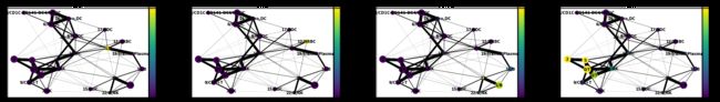
output_14_1.png
Annote groups with cell type
adata.obs['louvain'].cat.categories
Index(['0', '1', '2', '3', '4', '5', '6', '7', '8', '9', '10', '11', '12',
       '13', '14', '15', '16', '17', '18', '19', '20', '21', '22', '23'],
      dtype='object')
adata.obs['louvain_anno'] = adata.obs['louvain']
# annote them with names
adata.obs['louvain_anno'].cat.categories = ['0/T', '1/B', '2', '3/T', '4/MDDC', '5', '6/MDDC', '7/NK', '8/MDDC', '9/CD8+T', '10/NK', '11/B', '12/NRBC',
       '13', '14/CD1C-CD141-DC', '15/pDC', '16/Macro,DC', '17/pDC', '18/DC', '19/transB,Plasmab', '20','21','22/B,NK','23']
| Cluster | Cell Type | Marker Gene |
|---|---|---|
| 0 | T cell/IL-17Ralpha T cell | IL7R, CD3E, CD3D |
| 1 | B cell | MS4A1, CD79A |
| 2 | 高表达核糖体蛋白基因 | |
| 3 | CD8+ T cell, T helper, angiogenic T cell | CD3E, CXCR4, CD3D, CCL5, GZMK |
| 4 | Monocyte derived dendritic cell | S100A8, S100A9 |
| 5 | 高表达核糖体蛋白基因 | |
| 6 | Monocyte derived dendritic cell | S100A8, S100A9 |
| 7 | NK cell | PRF1, NKG7, KLRB1, KLRD1 |
| 8 | Monocyte derived dendritic cell | S100A8, S100A9 |
| 9 | CD8+ T cell | GZMK, CD3D, CD8A, NKG7 * |
| 10 | NK Cell | GNLY, NKG7, PTPRC |
| 11 | B cell | CD24, CD79A, CD37, CD79B |
| 12 | Red blood cell(Erythrocyte) | HBB, HBA1,GYPA |
| 13 | not known | |
| 14 | CD1C-CD141- dendritic cell | FCGR3A, CST3 |
| 15 | Plasmacytiod dendritic cell | HSP90B1, SSR4, PDIA4, SEC11C, MZB1, UBE2J1, FKBP2, DERL3, HERPUD1, ITM2C |
| 16 | Macrophage/ dendritic cell | LYZ, HLA-DQA1, AIF1, CD74, FCER1A, CST3 |
| 17 | Plasmacytiod dendritic cell | IRF8, TCF4, LILRA4 * |
| 18 | Megakaryocyte progenitor cell/Megakaryocyte | PF4, PPBP, / GP9 |
| 19 | transitional B cell / Plasmablast | CD24, CD79B |
| 20 | not known | |
| 21 | B cell | MS4A1, CD79A, CD37, CD74 |
| 22 | B cell , NK cell | CD74,CD79A, NKG7, GZMH |
| 23 | not known |
上面这个大家看看就好,我自己也不确定,请自行翻阅文献!!!
sc.tl.paga(adata, groups='louvain_anno')
running PAGA
    finished (0:00:13.55) --> added
    'paga/connectivities', connectivities adjacency (adata.uns)
    'paga/connectivities_tree', connectivities subtree (adata.uns)
sc.pl.paga(adata, threshold=0.03)
--> added 'pos', the PAGA positions (adata.uns['paga'])

output_21_1.png
adata
AnnData object with n_obs × n_vars = 315509 × 1314
    obs: 'n_genes', 'percent_mito', 'n_counts', 'louvain', 'louvain_anno'
    var: 'gene_ids', 'n_cells', 'highly_variable', 'means', 'dispersions', 'dispersions_norm'
    uns: 'louvain', 'louvain_colors', 'neighbors', 'pca', 'draw_graph', 'diffmap_evals', 'paga', 'louvain_sizes', 'louvain_anno_sizes', 'louvain_anno_colors'
    obsm: 'X_pca', 'X_umap', 'X_tsne', 'X_draw_graph_fa', 'X_diffmap'
    varm: 'PCs'
sc.tl.draw_graph(adata, init_pos='paga')
drawing single-cell graph using layout "fa"
    finished (1:03:55.77) --> added
    'X_draw_graph_fa', graph_drawing coordinates (adata.obsm)
Add pesudotime parameters
# the most primitive cell is refered as 0 persudotime.
# Group 13 is the nearest cell population to Hematopoietic stem cell.

adata.uns['iroot'] = np.flatnonzero(adata.obs['louvain_anno']  == '13')[0]
sc.tl.dpt(adata)
computing Diffusion Pseudotime using n_dcs=10
    finished (0:00:00.04) --> added
    'dpt_pseudotime', the pseudotime (adata.obs)
sc.pl.draw_graph(adata, color=['louvain_anno', 'dpt_pseudotime'],
                 legend_loc='right margin',title = ['','pseudotime'])

output_26_0.png
sc.pl.draw_graph(adata, color=['louvain_anno'],
                 legend_loc='right margin',title = ['']) #plot again to see full legends info

output_27_0.png
try other "iroot" setting
adata.uns['iroot'] = np.flatnonzero(adata.obs['louvain_anno']  == '5')[0]
sc.tl.dpt(adata)
sc.pl.draw_graph(adata, color=['louvain_anno', 'dpt_pseudotime'],
                 legend_loc='right margin',title = ['','pseudotime'])
computing Diffusion Pseudotime using n_dcs=10
    finished (0:00:00.04) --> added
    'dpt_pseudotime', the pseudotime (adata.obs)

output_29_1.png
Several other cell types are chosen to be "root" for diffusion pseudotime, however the pseudotime graphs look no big different.
..it doesn't look meaningful. didn't see any trajectory to describe cell development.
I think the "denoising graph" step is to blame. Will skip it next time.
Otherwise i should zoom it into a specific cell population, but have no idea which kind of cell i should choose...
Beautify the graphs
Choose the colors of the clusters a bit more consistently.
pl.figure(figsize=(8, 2))
for i in range(28):
    pl.scatter(i, 1, c=sc.pl.palettes.zeileis_26[i], s=200)
pl.show()

output_35_0.png
zeileis_colors = np.array(sc.pl.palettes.zeileis_26)
new_colors = np.array(adata.uns['louvain_anno_colors'])
new_colors[[13]] = zeileis_colors[[12]]  # Stem(?) colors / green
new_colors[[12]] = zeileis_colors[[5]]  # Ery colors / red
new_colors[[4,6,8,15,17]] = zeileis_colors[[17,17,17,16,16]]  # monocyte derived dendritic cell and pDC/ yellow
new_colors[[14,16,18]] = zeileis_colors[[16,16,16]]  # DC / yellow
new_colors[[0,3,9]] = zeileis_colors[[6,6,6]]  # T cell / light blue
new_colors[[7,10]] = zeileis_colors[[0,0]]  # NK cell / dark blue
new_colors[[1,11,22,19]] = zeileis_colors[[22,22,22,21]]  # B cell / pink
new_colors[[21,23,20]] = zeileis_colors[[25,25,25]]  # Not known / grey
new_colors[[2, 5]] = zeileis_colors[[25, 25]]  # outliers / grey
adata.uns['louvain_anno_colors'] = new_colors
adata
AnnData object with n_obs × n_vars = 315509 × 1314
    obs: 'n_genes', 'percent_mito', 'n_counts', 'louvain', 'louvain_anno', 'dpt_pseudotime'
    var: 'gene_ids', 'n_cells', 'highly_variable', 'means', 'dispersions', 'dispersions_norm'
    uns: 'louvain', 'louvain_colors', 'neighbors', 'pca', 'draw_graph', 'diffmap_evals', 'paga', 'louvain_sizes', 'louvain_anno_sizes', 'louvain_anno_colors', 'iroot'
    obsm: 'X_pca', 'X_umap', 'X_tsne', 'X_draw_graph_fa', 'X_diffmap'
    varm: 'PCs'
sc.pl.draw_graph(adata, color=['louvain_anno'],
                 legend_loc='right margin',title = [''])

output_40_0.png
this is a piece of shit.
screw it!!!!!