时序分析 21 高斯混合模型 （中）

时序分析 22 高斯混合模型 （中）

…接上

    金融时序经常呈现不平稳的状态，同时金融市场也会处于不同的阶段。例如牛市和熊市，高波动期/中波动期/低波动期。有时候市场价格和过去的价格是正相关的而有时是负相关的；有时和某些变量呈现线性关系而有时呈现非线性关系。

    我们在分析时序数据时，判断和预测市场所处的阶段非常重要。本系列文章前面所讨论的隐含马尔可夫模型就是对此类问题的一种方法，本篇文章着重讨论如何使用高斯混合模型来对时序数据分段。

    高斯混合模型的基本逻辑是假设每一个阶段是由高斯过程所产生，该过程的参数是可估计的。在这种假设下，GMM使用期望最大化方法(EM)来求得问题的最优解。

    下面我们就用实际的数据和例子来演示这个方法和过程，此例所要探究的市场阶段为平稳期(低波动律）和风险期(高波动率)。

导入包和确定工作环境

%load_ext watermark
%watermark

%load_ext autoreload
%autoreload 2

from IPython.display import display
from IPython.core.debugger import set_trace as bp
# import standard libs
from pathlib import PurePath, Path
import sys
import time
import os
import pickle
os.environ['THEANO_FLAGS'] = 'device=cpu,floatX=float32'

# get project dir
pp = PurePath(Path.cwd()).parts[:-1]
pdir = PurePath(*pp)
data_dir = pdir/'data'
script_dir = pdir / 'scripts' 
sys.path.append(script_dir.as_posix())

# import python scientific stack
import pandas as pd
pd.options.display.float_format = '{:,.4f}'.format
import pandas_datareader.data as web
import numpy as np
import sklearn.mixture as mix
from sklearn.model_selection import TimeSeriesSplit
import statsmodels.tsa.api as smt
import statsmodels.api as sm
import scipy.stats as stats
from numba import jit
import math
import pymc3 as pm
from theano import shared, theano as tt
from multiprocessing import cpu_count

# import visual tools
from mpl_toolkits import mplot3d
import matplotlib as mpl
import matplotlib.pyplot as plt
import matplotlib.gridspec as gridspec
%matplotlib inline
import plotnine as pn
import mizani.breaks as mzb
import mizani.formatters as mzf
import seaborn as sns
savefig_kwds=dict(dpi=300, bbox_inches='tight')
# import util libs
from tqdm import tqdm
import warnings
warnings.filterwarnings("ignore")
#from utils import cprint
import cprint
# set globals
plt.style.use('seaborn-talk')
plt.style.use('bmh')
plt.rcParams['font.family'] = 'Bitstream Vera Sans'#'DejaVu Sans Mono'
#plt.rcParams['font.size'] = 9.5
plt.rcParams['font.weight'] = 'medium'
plt.rcParams['figure.figsize'] = 10,7

blue, green, red, purple, gold, teal = sns.color_palette('colorblind', 6)
RANDOM_STATE = 777

print()
%watermark -p pandas,pandas_datareader,numpy,sklearn,statsmodels,scipy,pymc3,matplotlib,seaborn,plotnine

Last updated: 2020-12-20T18:17:08.204910+08:00

Python implementation: CPython
Python version : 3.7.3
IPython version : 7.4.0

Compiler : MSC v.1915 64 bit (AMD64)
OS : Windows
Release : 10
Machine : AMD64
Processor : Intel64 Family 6 Model 94 Stepping 3, GenuineIntel
CPU cores : 8
Architecture: 64bit

The autoreload extension is already loaded. To reload it, use:
%reload_ext autoreload

pandas : 1.1.5
pandas_datareader: 0.9.0
numpy : 1.16.2
sklearn : 0.20.3
statsmodels : 0.12.1
scipy : 1.2.1
pymc3 : 3.7
matplotlib : 3.3.3
seaborn : 0.9.0
plotnine : 0.7.1

我们先用测试数据试一下，

• 假设我们在分析三年的交易数据(252*3)
• 平稳期(stable)的收益均值为2.5%，波动率为9%
• 风险期收益均值为-1%，波动率为25%
• 平稳期和风险期出现的概率相同
      当然，我们知道以上的初始猜测是不太可能正确的。 下一步，我们利用高斯混合模型中的EM算法来进行测算，把概率或者权重分配给每一个数据点。 假如第一个数据点的收益为1.3%，我们计算平稳期(均值为2.5%，标准差为9%）的高斯分布产生这个数据点的概率。同样的过程应用于所有的数据点。然后再以类似的方式计算风险期产生这些数据点的概率。
      最后，我们加总这些概率，规范化，并且使用它们重新估算平稳期和风险期的均值和标准差。
      重复以上过程直到收敛

    在这个模拟的例子中，我们认为真实的均值、方差已知。我们只是验证GMM是否可以把真实的值挖掘出来。

生成假想数据

# Let's create some example return data to walk through the process. We will create a synthetic return series composed of two gaussians with different parameters. 
n = 252 * 7

true_stable_mu, true_stable_sigma = 0.15, 0.25
true_risky_mu, true_risky_sigma = -0.17, 0.45

true_prob_stable = 0.65
true_prob_risky = 1 - true_prob_stable

true_mus = np.array([true_stable_mu, true_risky_mu])
true_sigmas = np.array([true_stable_sigma, true_risky_sigma])
true_probs = np.array([true_prob_stable, true_prob_risky])

def mix_data(mus, sigmas, probs, n):

    np.random.seed(0)
    # randomly sample from binomial to select distr.
    z = np.random.binomial(1, true_probs[1], n)
    # sample from normal distr. and associated parameters according to z
    X = np.random.normal(true_mus[z], true_sigmas[z])
    
    # fake dates to make it look real
    fake_dates = pd.date_range('2011', periods=n)
    fake_returns = pd.Series(X, index=fake_dates)
    
    return fake_returns

mixed = mix_data(true_mus, true_sigmas, true_probs, n=n)

fig, axs = plt.subplots(nrows=3, figsize=(10,7))#, sharex=True)

mixed.plot(ax=axs[0], label='fake returns')
mixed.cumsum().plot(ax=axs[1], label='fake cumulative returns')
sns.distplot(mixed, ax=axs[2], kde_kws=dict(cut=0), label='fake kde returns')
for ax in axs: 
    ax.legend(loc='upper left') 
    ax.tick_params('both', direction='inout', length=7, width=1, which='major')
plt.tight_layout()

# code adapted from: https://github.com/sseemayer/mixem

class Normal:
    """Univariate normal distribution with parameters (mu, sigma)."""

    def __init__(self, mu, sigma):
        self.mu = mu
        self.sigma = sigma

    def log_density(self, data):
        """fn: compute log pdf of normal distr. given parameters and data"""
        
        assert(len(data.shape) == 1), "Expect 1D data!"
        
        # uncomment to confirm they produce same values
        log_pdf = stats.norm.logpdf(data, loc=self.mu, scale=self.sigma)
        #log_pdf = - (data - self.mu) ** 2 / (2 * self.sigma ** 2) - np.log(self.sigma) - 0.5 * np.log(2 * np.pi)
        return log_pdf

    def estimate_parameters(self, data, weights):
        """fn: estimate parameters of normal distr. given data and weights"""
        
        assert(len(data.shape) == 1), "Expect 1D data!"

        wsum = np.sum(weights)

        self.mu = np.sum(weights * data) / wsum
        self.sigma = np.sqrt(np.sum(weights * (data - self.mu) ** 2) / wsum)

初始化EM算法的参数

# terrible guesses at the true prior probability
init_stable_prob = 0.5
init_volatile_prob = 0.5

# guesses at starting mean
init_stable_mean = 0.10
init_volatile_mean = -0.1

# guesses at starting std
init_stable_std = 0.10
init_volatile_std = 0.3

init_probs = np.array([init_stable_prob, init_volatile_prob])
init_means = np.array([init_stable_mean, init_volatile_mean])
init_sigmas = np.array([init_stable_std, init_volatile_std])

现在我们可以实现算法的步骤

# wrap our distributions in a list
distributions = [Normal(init_means[0], init_sigmas[0]), 
                 Normal(init_means[1], init_sigmas[1])]
# set data
data = mixed.copy()    

# set algorithm parameters
max_iterations = tol_iters = 1000
tol=1e-5

# get key dim info
n_distr = true_mus.shape[0]
n_data = data.shape[0]

weight = np.array(init_probs) # init weight array
last_ll = np.full((tol_iters, ), np.nan) # init log-likelihood array
resp = np.empty((n_data, n_distr)) # init algo weights/resp array
log_density = np.empty((n_data, n_distr)) # init logpdf array

iteration = 0 # init counter

运行EM算法

while True:
    # ---------------------------------------------------------
    # E-step 
    # ---------------------------------------------------------
    
    # compute responsibilities aka weights
    for d in range(n_distr):
        log_density[:, d] = distributions[d].log_density(data)
        
    # normalize responsibilities of distributions so they sum up to one for example
    resp = weight[np.newaxis, :] * np.exp(log_density)
    resp /= np.sum(resp, axis=1)[:, np.newaxis]
    
    # compute log-likelihood
    log_likelihood = np.sum(resp @ log_density.T) # matrix multiplication
    
    # ---------------------------------------------------------
    # M-step 
    # ---------------------------------------------------------
    
    # now that we have the new weights we update the parameters
    # of the distributions
    for d in range(n_distr):
        distributions[d].estimate_parameters(data, resp[:, d])

    weight = np.mean(resp, axis=0)
    
    # ---------------------------------------------------------
    # check convergence
    # ---------------------------------------------------------
    
    if np.isnan(log_likelihood):
        last_ll[0] = log_likelihood
        print('loglk is nan')
        break
    
    if  ((last_ll[0] - log_likelihood) / last_ll[0]) <= tol:
        last_ll[0] = log_likelihood
        print('change in loglk less than tolerance')
        break

    if iteration >= max_iterations:
        last_ll[0] = log_likelihood
        print('reached maximum iterations')
        break

    # ---------------------------------------------------------
    # store value of current iteration in last_ll[0]
    #   and shift older values to the right
    # ---------------------------------------------------------    
    last_ll[1:] = last_ll[:-1]
    last_ll[0] = log_likelihood
    
    # ---------------------------------------------------------
    # info display
    # ---------------------------------------------------------    
    mus = np.array([distributions[i].mu for i in range(n_distr)])
    sigs = np.array([distributions[i].sigma for i in range(n_distr)])
    
    regime_map = {
     0:'stable', 1:'risky'}
    iter_data = (pd.DataFrame(np.vstack([mus, sigs, weight,
                                         true_mus, true_sigmas, true_probs]),
                              columns=[f'{regime_map[i]} regime' for i in range(n_distr)],
                              index=['means', 'sigmas', 'weights',
                                     'true_means', 'true_sigmas', 'true_weights'])
                 .round(3))
    
    if iteration % 50==0:
        print()
        print('-'*77)
        print(f'iteration: {iteration}')
        print(f"ll new: {last_ll[0].round(3)}")
        display(iter_data.T)
    iteration += 1      

---

_last_ll = last_ll[pd.notnull(last_ll)]
plt.plot(np.arange(0,len(_last_ll)), _last_ll[::-1])
plt.title('Maximizing Log Likelihood')

Text(0.5, 1.0, ‘Maximizing Log Likelihood’)

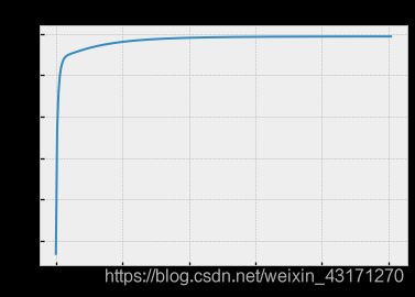
结果不错！我们通过这个假想例子证实了GMM+EM的有效性。

用真实数据

infp = "E:\datasets\etf_returns_ending_2017-12-31.parq"
R = (pd.read_parquet(infp,engine="fastparquet")).assign(year=lambda df: df.index.year)
R.head()

R.info()

sym = 'SPY' # example symbol
df = R.loc['2005':].copy() # use 2005 cutoff b/c it's first full year of data
df.info()

df2 = (df[[sym]]
       .assign(normal=lambda df:
               stats.norm.rvs(df[sym].mean(), df[sym].std(),
                                              size=len(df[sym])))
       .assign(laplace=lambda df: 
               stats.laplace.rvs(df[sym].mean(), df[sym].std(),
                                              size=len(df[sym]))))

df2.head()

p = (pn.ggplot(pd.melt(df2), pn.aes(x='value', color='variable'))
     +pn.geom_density(pn.aes(fill='variable'), alpha=0.5))
p.draw();

p = (pn.ggplot(pd.melt(df2), pn.aes(x='value', color='variable'))
     +pn.geom_histogram(pn.aes(y='..ndensity..', fill='variable'), alpha=0.5))
p.draw();

上图展示了以SPY的均值和方差为参数的正态分布和拉普拉斯分布于原数据的分布的比较。很明显，实际数据显现出了尖峰肥尾特征。

未完待续…