图像分类篇——使用pytorch搭建ResNet网络
目录
- 1. ResNet网络详解
-
- 1.1 ResNet网络概述
- 1.2 Batch Normalization
- 1.3 residual结构
- 1.4 ResNet结构和详细参数
- 1.5 迁移学习
- 2. Pytorch搭建
-
- 2.1 model.py
- 2.2 train.py
- 2.3 predict.py
本文为学习记录和备忘录,对代码进行了详细注释,以供学习。
内容来源:
★github: https://github.com/WZMIAOMIAO/deep-learning-for-image-processing
★b站:https://space.bilibili.com/18161609/channel/index
★CSDN:https://blog.csdn.net/qq_37541097
1. ResNet网络详解
1.1 ResNet网络概述
ResNet在2015年由微软实验室提出,斩获当年ImageNet竞赛中分类任务第一名,目标检测第一名。获得COCO数据集中目标检测第一名,图像分割第一名。
论文全称:Deep Residual Learining for Image Recognition
论文链接:Deep Residual Learining for Image Recognition
网络的亮点:
★超深的网络结构(突破1000层)
★提出residual模块
★使用Batch Normalization加速训练(丢弃dropout)
问题背景:
▲单纯地将卷积层和池化层叠加也能得到超深的网络结构,但是随着网络层数的不断加深,梯度消失或梯度爆炸问题会越发严重。
梯度消失:假设每一层的误差梯度是1个小于1的数,则在反向传播的过程中,每向前传播1次,都要乘以1个小于1的误差梯度,当网络越来越深时,梯度会越来越小,结果会更加趋于0,即梯度消失现象。
梯度爆炸:假设每一层的误差梯度都是1个大于1的数,则在反向传播的过程中,每向前传播1次,都要乘以1个大于1的误差梯度,当网络越来越深时,梯度会越来越大,即梯度爆炸现象。
通常通过对数据的标准化处理、权重初始化以及Batch Normalization来解决梯度消失或梯度爆炸问题。
▲在解决了梯度消失或梯度爆炸问题后,仍然会存在层数很深时没有层数少时效果好的问题,原文中将这个问题称为“退化问题(degradation problem)”,解决这个问题的方法是引入“残差模块(Residual Module)”。
1.2 Batch Normalization
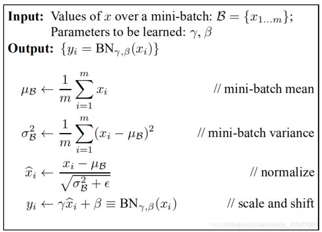
Batch Normalization的目的是使我们的一批(Batch)feature map满足均值为0,方差为1的分布规律。其中 μ 和 σ² 是在正向传播过程中统计得到的, γ 和 β 是在反向传播过程中训练得到。
对于batch normalization的详细讲解可见:Batch Normalization详解以及pytorch实验
1.3 residual结构

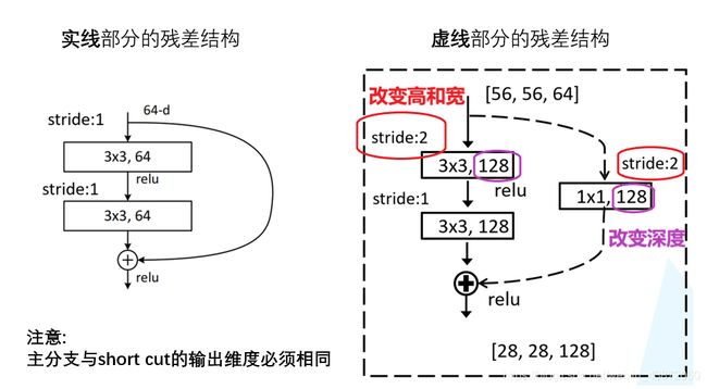
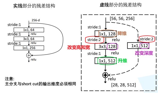
- 对于网络层数较少的,用左边这个残差结构,具体用于ResNet-18/34。而右边这个结构用于ResNet-50/101/152。右边和左边比起来主要区别在于输入和输出加上了1×1的卷积层,第1个1×1的卷积层起降维的作用,第2个1×1的卷积层起升维的作用。
- 主分支上经过一系列卷积层之后得到的特征矩阵与输入特征矩阵进行相加,相加之后再通过relu函数,注意主分支经过相加之前的那一个卷积层后没有经过relu函数,而是和输入矩阵相加后才通过relu函数。(这里的相加不同于VGG网络中在channel维度上进行拼接)
并且主分支与侧分支(short cut)的输出特征矩阵的shape必须相同,即height,width,channel相同。
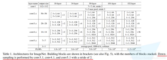
1.4 ResNet结构和详细参数
以ResNet-34为例,其结构如下:
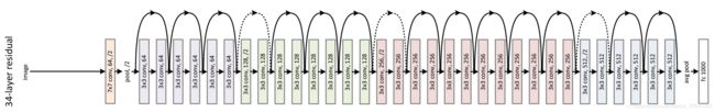
在结构图中,有的残差结构是实线,有的残差结构是虚线。实线残差结构的输入特征矩阵和输出特征矩阵的shape是完全相同的,故它们能直接相加。而虚线残差结构输入特征矩阵和输出特征矩阵的shape是不同的,它能够将输入矩阵的高、宽、深度全部改变。它们的区别如下:
- 主分支中3×3卷积层的步距发生了变化,因为需要将输入特征矩阵的height和width变小,如从56变为28,这可由stride=2来实现,然后通过128个卷积核来改变特征矩阵深度channel。
- 在short cut中,通过stride=2改变height和width,如从56变为28,在通过1×1卷积改变特征矩阵的channel,如用128个1×1个卷积核将特征矩阵深度从64变为128。这样就能保证在主分支和short cut分支中得到的2个特征矩阵的shape相同。
具体地:
用于ResNet-18/34:

用于ResNet-50/101/152:

注:对于ResNet-18/34,conv2的第1层卷积层为实线残差结构,conv3/4/5的第1层卷积层为虚线残差结构。而对于ResNet-50/101/152,conv2的第1层卷积层为特殊虚线残差结构,conv3/4/5的第1层卷积层为虚线残差结构。特殊虚线残差结构的特殊在于,它只改变输入特征矩阵的深度,不改变其高和宽,达到这个目的的方法是使stride=1。
1.5 迁移学习
随着卷积层层数的加深,每个卷积层学到的信息越来越复杂,越来越抽象。将学习好的网络的浅层网络的一些参数迁移到新的网络中来,新的网络也拥有了识别底层通用特征的能力,新的网络就能够更加快速地去学习新的数据集的高维特征。
使用迁移学习的优势:
- 能够快速的训练出一个理想的结果。
- 当数据集较小时也能训练出理想的效果。
常见的迁移学习方式:
- 载入权重后训练所有参数。
- 载入权重后只训练最后几层参数。
- 载入权重后在原网络基础上再添加一层全连接层,仅训练最后一个全连接层。
2. Pytorch搭建
对于代码的解释都在注释中,方便对照查看学习。
2.1 model.py
无论是18层的网络、34层的网络、50层的网络、101层的网络还是152层的网络,它们的网络框架基本相同:首先通过1个7×7的卷积层,然后通过1个3×3的最大池化下采样,然后通过conv2所对应的一系列残差结构、conv3所对应的一系列残差结构、conv4所对应的一系列残差结构和conv5所对应的一系列残差结构,最后通过平均池化下采样以及全连接输出层。
(1)先定义18/34 layers网络的残差结构,对照着实线和虚线的残差结构图,定义一个类class BasicBlock(nn.Module):
- 要点1:观察上图,18层和34层网络残差结构中,主分支采用的卷积核个数有没有发生变化,即第1层和第2层卷积核个数相同,此处设置expansion = 1。
- 要点2:比较残差结构的第1层卷积层,实线残差结构步距为1,虚线残差结构步距为2,通过传入参数stride=stride控制步距的改变(对应下述代码1)。而在残差结构的第2层卷积层中,不管实线还是虚线残差结构,第2层卷积层的步距都为1,故传入参数stride=1(对应下述代码2)。即:
self.conv1 = nn.Conv2d(in_channels=in_channel, out_channels=out_channel, kernel_size=3, stride=stride, padding=1, bias=False)
self.conv2 = nn.Conv2d(in_channels=out_channel, out_channels=out_channel, kernel_size=3, stride=1, padding=1, bias=False)
- 要点3:使用BN时,卷积中的参数bias设置为False;且BN层放在conv层和relu层中间。BN层的输入为卷积层输出特征矩阵深度。
- 要点4:在正向传播过程中,如果初始化传入参数downsample=None的话,即为实线残差结构,将输入特征矩阵x赋给short cut分支上作为输出值;如果self.downsample is not None,则为虚线残差结构,需要将输入特征矩阵x赋给下采样函数,得到的结果作为short cut分支的结果。即:
identity = x
        if self.downsample is not None:
            identity = self.downsample(x)
- 要点5:对于卷积层第1层的卷积结果,通过BN层后经过relu函数,但是卷积层第2层结果通过BN层后不直接通过relu函数,而是与short cut分支结果相加后再经过relu函数。即:
out = self.bn2(out)
out += identity
out = self.relu(out)
(2)然后定义50/101/152layers网络的残差结构,对照着实线和虚线的残差结构图,定义一个类class Bottleneck(nn.module):
定义18层,34层网络的残差结构中所讲述的所有要点在定义更深层次的残差结构是都需要注意。
- 要点1:但在定义expansion的值时有所不同:在50层、101层和152层的残差结构中,第1层和第2层卷积核个数相同,第3层的卷积核个数是第1层、第2层的4倍,这里设置expansion = 4。在定义第3层卷积层时,卷积核个数out_channels=out_channel*self.expansion。即:
self.conv3 = nn.Conv2d(in_channels=width, out_channels=out_channel*self.expansion, kernel_size=1, stride=1, bias=False)=

self.bn3 = nn.BatchNorm2d(out_channel*self.expansion)
(3)定义ResNet整个网络的框架部分:
- 要点1:初始化函数传入的参数。
def __init__(self, block, blocks_num, num_classes=1000, include_top=True, groups=1, width_per_group=64):
block对应的是残差结构,根据不同的层结构传入不同的block,如定义18或34层网络结构,这里的block即为BasicBlock,若为50或101或152层网络,则block为Bottleneck。blocks_num为所使用残差结构的数目,这是一个列表参数,如对应34层而言,blocks_num即为[3,4,6,3]。num_classes指训练集的分类个数,include_top是为了方便在ResNet基础上搭建更复杂的网络。
- 要点2:通过定义make_layer函数生成每一部分残差结构。
需要注意的是,对于ResNet-18/34,conv2的第1层卷积层为实线残差结构,conv3/4/5的第1层卷积层为虚线残差结构。而对于ResNet-50/101/152,conv2的第1层卷积层为特殊虚线残差结构,conv3/4/5的第1层卷积层为虚线残差结构。特殊虚线残差结构的特殊在于,它只改变输入特征矩阵的深度,不改变其高和宽,达到这个目的的方法是使stride=1。
其详细原理和过程见下列代码及注释:
    def _make_layer(self, block, channel, block_num, stride=1):
        # block即残差结构BasicBlock或Bottleneck;channel是残差结构中卷积层所使用卷积核的个数(对应第1层卷积核个数)
        # block_num指该层一共包含了多少个残差结构
        downsample = None
        # 对于第1层而言,没有输入stride,默认等于1;对于18层或34层网络而言,由于expansion=1,则in_channel=channel*expansion,不执行下列if语句
        # 而对于50,101,152层网络而言,expansion=4,in_channel!=channel*expansion,会执行下面的if语句
        # 但从第2层开始,stride=2,不论多少层的网络,都会生成虚线残差结构
        if stride != 1 or self.in_channel != channel * block.expansion:
            downsample = nn.Sequential(  # 定义下采样函数
                nn.Conv2d(self.in_channel, channel * block.expansion, kernel_size=1, stride=stride, bias=False),
                # 而对于50,101,152层网络而言,在conv2所对应的一系列残差结构的第1层中,虽然是虚线残差结构,但是只需要调整特征矩阵深度,因此第1层默认stride=1
                # 而对于cmv3,cnv4,conv5,不仅调整深度,还要将高和宽缩小为一半,因此在layer2,layer3,layer4中需要传入参数stride=2
                # 输出特征矩阵深度为channel * block.expansion
                nn.BatchNorm2d(channel * block.expansion))  # 对应的BN层传入的特征矩阵深度为channel * block.expansion

        layers = []  # 定义1个空列表
        # 因为不同深度的网络残差结构中的第1层卷积层操作不同,故需要分而治之
        layers.append(block(self.in_channel, channel, downsample=downsample, stride=stride, groups=self.groups,
                            width_per_group=self.width_per_group))
        # 首先将第1层残差结构添加进去,block即BasicBlock或Bottleneck,传入参数有输入特征矩阵深度self.in_channel(64),
        # 残差结构所对应主分支上第1层卷积层的卷积核个数channel,定义的下采样函数和stride参数
        # 对于18/34layers网络,第一层残差结构为实线结构,downsample=None;
        # 对50/101/152layers的网络,第一层残差结构为虚线结构,将特征矩阵的深度翻4倍,高和宽不变。且对于layer1而言,stride=1
        self.in_channel = channel * block.expansion
        # 对于18/34layers网络,expansion=1,输出深度不变;对于50/101/152layers的网络,expansion=4,输出深度翻4倍。

        for _ in range(1, block_num):
            layers.append(block(self.in_channel, channel, groups=self.groups, width_per_group=self.width_per_group))
        # 通过循环,将剩下一系列的实线残差结构压入layers[],不管是18/34/50/101/152layers,从它们的第2层开始,全都是实线残差结构。
        # 注意循环从1开始,因为第1层已经搭接好。传入输入特征矩阵深度和残差结构第1层卷积核个数
        return nn.Sequential(*layers)  # 构建好layers[]列表后,通过非关键字参数的形式传入到nn.Sequential,将定义的一系列层结构组合在一起并返回得到layer1
然后在初始化函数中通过以下语句生成不同层的一系列残差结构:
        self.layer1 = self._make_layer(block, 64, blocks_num[0])  # layer1对应表格中conv2所包含的一系列残差结构
        self.layer2 = self._make_layer(block, 128, blocks_num[1], stride=2)  # layer2对应表格中conv3所包含的一系列残差结构
        self.layer3 = self._make_layer(block, 256, blocks_num[2], stride=2)  # layer3对应表格中conv4所包含的一系列残差结构
        self.layer4 = self._make_layer(block, 512, blocks_num[3], stride=2)  # layer4对应表格中conv5所包含的一系列残差结构
模型部分全部代码如下:
import torch.nn as nn
import torch


class BasicBlock(nn.Module):  # 针对18层和34层的残差结构
    expansion = 1  # 对应着残差结构中主分支采用的卷积核个数有没有发生变化,18层和34层残差结构中,第1层和第2层卷积核个数相同,此处设置expansion = 1

    def __init__(self, in_channel, out_channel, stride=1, downsample=None, **kwargs):
        # 在初始化函数中传入以下参数:输入特征矩阵深度、输出特征矩阵深度(即主分支上卷积核个数),步距默认取1,下采样参数默认设置为None(其对应虚线残差结构)
        super(BasicBlock, self).__init__()
        self.conv1 = nn.Conv2d(in_channels=in_channel, out_channels=out_channel,
                               kernel_size=3, stride=stride, padding=1, bias=False)
        # 第1层卷积层,实线结构步距为1,虚线结构步距为2,通过传入参数stride=stride控制
        self.bn1 = nn.BatchNorm2d(out_channel)
        # 使用BN时,卷积中的参数bias设置为False;且BN层放在conv层和relu层中间。BN层的输入为卷积层输出特征矩阵深度。
        self.relu = nn.ReLU()
        self.conv2 = nn.Conv2d(in_channels=out_channel, out_channels=out_channel,
                               kernel_size=3, stride=1, padding=1, bias=False)
        # 不管实线还是虚线残差结构,第2层卷积层的步距都为1,故传入参数stride=1
        self.bn2 = nn.BatchNorm2d(out_channel)
        self.downsample = downsample  # 定义下采样方法

    def forward(self, x):
        identity = x  # 将输入特征矩阵x赋给short cut分支上作为输出值(这是下采样函数等于None,即实线结构的情况)
        if self.downsample is not None:  # 如果下采样函数不等于None的话,即是虚线结构的情况
            identity = self.downsample(x)  # 将输入特征矩阵x赋给下采样函数,得到的结果作为short cut分支的结果

        # 主支线
        out = self.conv1(x)
        out = self.bn1(out)
        out = self.relu(out)

        out = self.conv2(out)
        out = self.bn2(out)  # 注意这里不经过relu函数,需要将这里的输出和short cut支线的输出相加再经过relu函数

        out += identity  # 主分支输出与short cut分支输出相加
        out = self.relu(out)

        return out


class Bottleneck(nn.Module):
    """
    注意:原论文中,在虚线残差结构的主分支上,第一个1x1卷积层的步距是2,第二个3x3卷积层步距是1。
    但在pytorch官方实现过程中是第一个1x1卷积层的步距是1,第二个3x3卷积层步距是2,
    这么做的好处是能够在top1上提升大概0.5%的准确率。
    可参考Resnet v1.5 https://ngc.nvidia.com/catalog/model-scripts/nvidia:resnet_50_v1_5_for_pytorch
    """
    expansion = 4  # 在50层、101层和152层的残差结构中,第1层和第2层卷积核个数相同,第3层的卷积核个数是第1层、第2层的4倍,这里设置expansion = 4

    def __init__(self, in_channel, out_channel, stride=1, downsample=None,
                 groups=1, width_per_group=64):
        super(Bottleneck, self).__init__()

        width = int(out_channel * (width_per_group / 64.)) * groups

        self.conv1 = nn.Conv2d(in_channels=in_channel, out_channels=width,
                               kernel_size=1, stride=1, bias=False)  # squeeze channels
        # 无论实线结构还是虚线结构,第1层卷积层都是kernel_size=1, stride=1
        self.bn1 = nn.BatchNorm2d(width)
        # -----------------------------------------
        self.conv2 = nn.Conv2d(in_channels=width, out_channels=width, groups=groups,
                               kernel_size=3, stride=stride, bias=False, padding=1)
        # 实线残差结构第2层3×3卷积stride=1,而虚线残差结构第2层3×3卷积stride=2,因此出入参数stride=stride
        self.bn2 = nn.BatchNorm2d(width)
        # -----------------------------------------
        self.conv3 = nn.Conv2d(in_channels=width, out_channels=out_channel*self.expansion,
                               kernel_size=1, stride=1, bias=False)  # unsqueeze channels
        # 第3层卷积层步距都为1,但是第3层卷积核个数为第1层和第2层卷积核个数的4倍,则卷积核个数out_channels=out_channel*self.expansion
        self.bn3 = nn.BatchNorm2d(out_channel*self.expansion)  # BN层输入卷积层深度等于卷积层3输出特征矩阵的深度
        self.relu = nn.ReLU(inplace=True)
        self.downsample = downsample

    def forward(self, x):
        identity = x  # 将输入特征矩阵x赋给short cut分支上作为输出值(这是下采样函数等于None,即实线结构的情况)
        if self.downsample is not None:  # 如果下采样函数不等于None的话,即是虚线结构的情况
            identity = self.downsample(x)  # 将输入特征矩阵x赋给下采样函数,得到的结果作为short cut分支的结果

        out = self.conv1(x)
        out = self.bn1(out)
        out = self.relu(out)

        out = self.conv2(out)
        out = self.bn2(out)
        out = self.relu(out)

        out = self.conv3(out)
        out = self.bn3(out)  # 注意这里同样不经过relu函数,需要将这里的输出和short cut支线的输出相加再经过relu函数

        out += identity
        out = self.relu(out)

        return out


# 定义ResNet整个网络的框架部分
class ResNet(nn.Module):

    def __init__(self, block, blocks_num, num_classes=1000, include_top=True, groups=1, width_per_group=64):
        # block对应的是残差结构,根据不同的层结构传入不同的block,如定义18或34层网络结构,这里的block即为BasicBlock,若50,101,152,则block为Bottleneck
        # blocks_num为所使用残差结构的数目,这是一个列表参数,如对应34层而言,blocks_num即为[3,4,6,3]
        # num_classes指训练集的分类个数,include_top是为了方便在ResNet基础上搭建更复杂的网络
        super(ResNet, self).__init__()
        self.include_top = include_top
        self.in_channel = 64  # 输入特征矩阵深度,对应表格中maxpool后的特征矩阵深度,都是64

        self.groups = groups
        self.width_per_group = width_per_group

        self.conv1 = nn.Conv2d(3, self.in_channel, kernel_size=7, stride=2,
                               padding=3, bias=False)  # 对应表格中的7×7卷积层,输入特征矩阵(rgb图像)深度为3,stride=2,bias=False
        self.bn1 = nn.BatchNorm2d(self.in_channel)
        self.relu = nn.ReLU(inplace=True)
        self.maxpool = nn.MaxPool2d(kernel_size=3, stride=2, padding=1)  # 对应表格第2层,最大池化下采样
        self.layer1 = self._make_layer(block, 64, blocks_num[0])  # layer1对应表格中conv2所包含的一系列残差结构
        self.layer2 = self._make_layer(block, 128, blocks_num[1], stride=2)  # layer2对应表格中conv3所包含的一系列残差结构
        self.layer3 = self._make_layer(block, 256, blocks_num[2], stride=2)  # layer3对应表格中conv4所包含的一系列残差结构
        self.layer4 = self._make_layer(block, 512, blocks_num[3], stride=2)  # layer4对应表格中conv5所包含的一系列残差结构
        if self.include_top:
            self.avgpool = nn.AdaptiveAvgPool2d((1, 1))  # output size = (1, 1),自适应平均池化下采样
            self.fc = nn.Linear(512 * block.expansion, num_classes)

        for m in self.modules():  # 初始化操作
            if isinstance(m, nn.Conv2d):
                nn.init.kaiming_normal_(m.weight, mode='fan_out', nonlinearity='relu')

    def _make_layer(self, block, channel, block_num, stride=1):
        # block即残差结构BasicBlock或Bottleneck;channel是残差结构中卷积层所使用卷积核的个数(对应第1层卷积核个数)
        # block_num指该层一共包含了多少个残差结构
        downsample = None
        # 对于第1层而言,没有输入stride,默认等于1;对于18层或34层网络而言,由于expansion=1,则in_channel=channel*expansion,不执行下列if语句
        # 而对于50,101,152层网络而言,expansion=4,in_channel!=channel*expansion,会执行下面的if语句
        # 但从第2层开始,stride=2,不论多少层的网络,都会生成虚线残差结构
        if stride != 1 or self.in_channel != channel * block.expansion:
            downsample = nn.Sequential(  # 定义下采样函数
                nn.Conv2d(self.in_channel, channel * block.expansion, kernel_size=1, stride=stride, bias=False),
                # 而对于50,101,152层网络而言,在conv2所对应的一系列残差结构的第1层中,虽然是虚线残差结构,但是只需要调整特征矩阵深度,因此第1层默认stride=1
                # 而对于cmv3,cnv4,conv5,不仅调整深度,还要将高和宽缩小为一半,因此在layer2,layer3,layer4中需要传入参数stride=2
                # 输出特征矩阵深度为channel * block.expansion
                nn.BatchNorm2d(channel * block.expansion))  # 对应的BN层传入的特征矩阵深度为channel * block.expansion

        layers = []  # 定义1个空列表
        # 因为不同深度的网络残差结构中的第1层卷积层操作不同,故需要分而治之
        layers.append(block(self.in_channel, channel, downsample=downsample, stride=stride, groups=self.groups,
                            width_per_group=self.width_per_group))
        # 首先将第1层残差结构添加进去,block即BasicBlock或Bottleneck,传入参数有输入特征矩阵深度self.in_channel(64),
        # 残差结构所对应主分支上第1层卷积层的卷积核个数channel,定义的下采样函数和stride参数
        # 对于18/34layers网络,第一层残差结构为实线结构,downsample=None;
        # 对50/101/152layers的网络,第一层残差结构为虚线结构,将特征矩阵的深度翻4倍,高和宽不变。且对于layer1而言,stride=1
        self.in_channel = channel * block.expansion
        # 对于18/34layers网络,expansion=1,输出深度不变;对于50/101/152layers的网络,expansion=4,输出深度翻4倍。

        for _ in range(1, block_num):
            layers.append(block(self.in_channel, channel, groups=self.groups, width_per_group=self.width_per_group))
        # 通过循环,将剩下一系列的实线残差结构压入layers[],不管是18/34/50/101/152layers,从它们的第2层开始,全都是实线残差结构。
        # 注意循环从1开始,因为第1层已经搭接好。传入输入特征矩阵深度和残差结构第1层卷积核个数
        return nn.Sequential(*layers)  # 构建好layers[]列表后,通过非关键字参数的形式传入到nn.Sequential,将定义的一系列层结构组合在一起并返回得到layer1

    def forward(self, x):
        x = self.conv1(x)
        x = self.bn1(x)  # BN层位于卷积层和relu函数中间
        x = self.relu(x)
        x = self.maxpool(x)

        x = self.layer1(x)  # conv2对应的一系列残差结构
        x = self.layer2(x)  # conv3对应的一系列残差结构
        x = self.layer3(x)  # conv4对应的一系列残差结构
        x = self.layer4(x)  # conv5对应的一系列残差结构

        if self.include_top:
            x = self.avgpool(x)  # 平均池化下采样
            x = torch.flatten(x, 1)  # 展平处理
            x = self.fc(x)  # 全连接

        return x


def resnet34(num_classes=1000, include_top=True):
    # https://download.pytorch.org/models/resnet34-333f7ec4.pth
    return ResNet(BasicBlock, [3, 4, 6, 3], num_classes=num_classes, include_top=include_top)
    # 对于resnet34,block选用BasicBlock,残差层个数分别是[3,4,6,3]。如果是resnet18,则为[2,2,2,2]


def resnet50(num_classes=1000, include_top=True):
    # https://download.pytorch.org/models/resnet50-19c8e357.pth
    return ResNet(Bottleneck, [3, 4, 6, 3], num_classes=num_classes, include_top=include_top)
    # 对于resnet50,block选用Bottleneck,残差层个数分别是[3,4,6,3]。

def resnet101(num_classes=1000, include_top=True):
    # https://download.pytorch.org/models/resnet101-5d3b4d8f.pth
    return ResNet(Bottleneck, [3, 4, 23, 3], num_classes=num_classes, include_top=include_top)


def resnext50_32x4d(num_classes=1000, include_top=True):
    # https://download.pytorch.org/models/resnext50_32x4d-7cdf4587.pth
    groups = 32
    width_per_group = 4
    return ResNet(Bottleneck, [3, 4, 6, 3],
                  num_classes=num_classes,
                  include_top=include_top,
                  groups=groups,
                  width_per_group=width_per_group)


def resnext101_32x8d(num_classes=1000, include_top=True):
    # https://download.pytorch.org/models/resnext101_32x8d-8ba56ff5.pth
    groups = 32
    width_per_group = 8
    return ResNet(Bottleneck, [3, 4, 23, 3],
                  num_classes=num_classes,
                  include_top=include_top,
                  groups=groups,
                  width_per_group=width_per_group)
2.2 train.py
基本上与AlexNet,VGG,GoogLeNet相似,不同在于:
(1)图像预处理方式不同,一是对图片进行标准化处理的参数不同,这里的参数来自官网,二是对于验证集的图片,将原图片的长宽比固定不变,将其最小边长缩放到256,再使用中心裁剪裁剪一个224×224大小的图片。(原来的方式是直接resize成224×224)即:
    data_transform = {

        "train": transforms.Compose([transforms.RandomResizedCrop(224),
                                     transforms.RandomHorizontalFlip(),
                                     transforms.ToTensor(),
                                     transforms.Normalize([0.485, 0.456, 0.406], [0.229, 0.224, 0.225])]),  # 标准化参数来自官网
        "val": transforms.Compose([transforms.Resize(256),  # 验证过程图像预处理有变动,将原图片的长宽比固定不动,将其最小边长缩放到256
                                   transforms.CenterCrop(224),  # 再使用中心裁剪裁剪一个224×224大小的图片
                                   transforms.ToTensor(),
                                   transforms.Normalize([0.485, 0.456, 0.406], [0.229, 0.224, 0.225])])}
(2)采用预训练模型权重文件进行迁移学习。即:
    net = resnet34()
    # load pretrain weights
    # download url: https://download.pytorch.org/models/resnet34-333f7ec4.pth
    model_weight_path = "./resnet34-pre.pth"  # 保存权重的路径
    assert os.path.exists(model_weight_path), "file {} does not exist.".format(model_weight_path)
    net.load_state_dict(torch.load(model_weight_path, map_location=device))  # 通过net.load_state_dict方法载入模型权重
    # for param in net.parameters():
    #     param.requires_grad = False

    # change fc layer structure
    in_channel = net.fc.in_features  # net.fc即model.py中定义的网络的全连接层,in_features是输入特征矩阵的深度
    net.fc = nn.Linear(in_channel, 5)  # 重新定义全连接层,输入深度即上面获得的输入特征矩阵深度,类别为当前预测的花分类数据集类别5
    net.to(device)
训练部分全部代码如下:
import os
import json

import torch
import torch.nn as nn
import torch.optim as optim
from torchvision import transforms, datasets
from tqdm import tqdm

from model import resnet34


#  ####基本上与AlexNet,VGG,GoogLeNet相似,不同在于1.图像预处理line18-line26,2.采用预训练模型权重文件进行迁移学习line64-line73
def main():
    device = torch.device("cuda:0" if torch.cuda.is_available() else "cpu")
    print("using {} device.".format(device))

    data_transform = {

        "train": transforms.Compose([transforms.RandomResizedCrop(224),
                                     transforms.RandomHorizontalFlip(),
                                     transforms.ToTensor(),
                                     transforms.Normalize([0.485, 0.456, 0.406], [0.229, 0.224, 0.225])]),  # 标准化参数来自官网
        "val": transforms.Compose([transforms.Resize(256),  # 验证过程图像预处理有变动,将原图片的长宽比固定不动,将其最小边长缩放到256
                                   transforms.CenterCrop(224),  # 再使用中心裁剪裁剪一个224×224大小的图片
                                   transforms.ToTensor(),
                                   transforms.Normalize([0.485, 0.456, 0.406], [0.229, 0.224, 0.225])])}

    data_root = os.path.abspath(os.path.join(os.getcwd(), "../.."))  # get data root path
    image_path = os.path.join(data_root, "data_set", "flower_data")  # flower data set path
    assert os.path.exists(image_path), "{} path does not exist.".format(image_path)
    train_dataset = datasets.ImageFolder(root=os.path.join(image_path, "train"),
                                         transform=data_transform["train"])
    train_num = len(train_dataset)

    # {'daisy':0, 'dandelion':1, 'roses':2, 'sunflower':3, 'tulips':4}
    flower_list = train_dataset.class_to_idx
    cla_dict = dict((val, key) for key, val in flower_list.items())
    # write dict into json file
    json_str = json.dumps(cla_dict, indent=4)
    with open('class_indices.json', 'w') as json_file:
        json_file.write(json_str)

    batch_size = 16
    nw = min([os.cpu_count(), batch_size if batch_size > 1 else 0, 8])  # number of workers
    print('Using {} dataloader workers every process'.format(nw))

    train_loader = torch.utils.data.DataLoader(train_dataset,
                                               batch_size=batch_size, shuffle=True,
                                               num_workers=nw)

    validate_dataset = datasets.ImageFolder(root=os.path.join(image_path, "val"),
                                            transform=data_transform["val"])
    val_num = len(validate_dataset)
    validate_loader = torch.utils.data.DataLoader(validate_dataset,
                                                  batch_size=batch_size, shuffle=False,
                                                  num_workers=nw)

    print("using {} images for training, {} images for validation.".format(train_num,
                                                                           val_num))

    net = resnet34()
    # load pretrain weights
    # download url: https://download.pytorch.org/models/resnet34-333f7ec4.pth
    model_weight_path = "./resnet34-pre.pth"  # 保存权重的路径
    assert os.path.exists(model_weight_path), "file {} does not exist.".format(model_weight_path)
    net.load_state_dict(torch.load(model_weight_path, map_location=device))  # 通过net.load_state_dict方法载入模型权重
    # for param in net.parameters():
    #     param.requires_grad = False

    # change fc layer structure
    in_channel = net.fc.in_features  # net.fc即model.py中定义的网络的全连接层,in_features是输入特征矩阵的深度
    net.fc = nn.Linear(in_channel, 5)  # 重新定义全连接层,输入深度即上面获得的输入特征矩阵深度,类别为当前预测的花分类数据集类别5
    net.to(device)

    # define loss function
    loss_function = nn.CrossEntropyLoss()

    # construct an optimizer
    params = [p for p in net.parameters() if p.requires_grad]
    optimizer = optim.Adam(params, lr=0.0001)

    epochs = 3
    best_acc = 0.0
    save_path = './resNet34.pth'
    train_steps = len(train_loader)
    for epoch in range(epochs):
        # train
        net.train()  # 在训练过程中,self.training=True,有BN层的存在,区别于net.eval()
        running_loss = 0.0
        train_bar = tqdm(train_loader)
        for step, data in enumerate(train_bar):
            images, labels = data
            optimizer.zero_grad()
            logits = net(images.to(device))
            loss = loss_function(logits, labels.to(device))  # 计算损失
            loss.backward()  # 将损失反向传播
            optimizer.step()  # 更新每一个节点的参数

            # print statistics
            running_loss += loss.item()

            train_bar.desc = "train epoch[{}/{}] loss:{:.3f}".format(epoch + 1,
                                                                     epochs,
                                                                     loss)

        # validate
        net.eval()  # 在验证过程中,self.training=False,没有BN层
        acc = 0.0  # accumulate accurate number / epoch
        with torch.no_grad():  # 用以禁止pytorch对参数进行跟踪,即在验证过程中不去计算损失梯度
            val_bar = tqdm(validate_loader)
            for val_data in val_bar:
                val_images, val_labels = val_data
                outputs = net(val_images.to(device))
                # loss = loss_function(outputs, test_labels)
                predict_y = torch.max(outputs, dim=1)[1]
                acc += torch.eq(predict_y, val_labels.to(device)).sum().item()

                val_bar.desc = "valid epoch[{}/{}]".format(epoch + 1,
                                                           epochs)

        val_accurate = acc / val_num
        print('[epoch %d] train_loss: %.3f  val_accuracy: %.3f' %
              (epoch + 1, running_loss / train_steps, val_accurate))

        if val_accurate > best_acc:
            best_acc = val_accurate
            torch.save(net.state_dict(), save_path)

    print('Finished Training')


if __name__ == '__main__':
    main()
2.3 predict.py
需要注意的是,采用和训练方法一样的图像标准化处理,两者标准化参数相同。
预测部分全部代码如下:
import os
import json

import torch
from PIL import Image
from torchvision import transforms
import matplotlib.pyplot as plt

from model import resnet34


def main():
    device = torch.device("cuda:0" if torch.cuda.is_available() else "cpu")

    data_transform = transforms.Compose(
        [transforms.Resize(256),
         transforms.CenterCrop(224),
         transforms.ToTensor(),
         transforms.Normalize([0.485, 0.456, 0.406], [0.229, 0.224, 0.225])])  # 采用和训练方法一样的图像标准化处理,两者标准化参数相同。

    # load image
    img_path = "../tulip.jpg"
    assert os.path.exists(img_path), "file: '{}' dose not exist.".format(img_path)
    img = Image.open(img_path)
    plt.imshow(img)
    # [N, C, H, W]
    img = data_transform(img)
    # expand batch dimension
    img = torch.unsqueeze(img, dim=0)

    # read class_indict
    json_path = './class_indices.json'
    assert os.path.exists(json_path), "file: '{}' dose not exist.".format(json_path)

    json_file = open(json_path, "r")
    class_indict = json.load(json_file)

    # create model
    model = resnet34(num_classes=5).to(device)  # 实例化模型时,将数据集分类个数赋给num_classes并传入模型

    # load model weights
    weights_path = "./resNet34.pth"
    assert os.path.exists(weights_path), "file: '{}' dose not exist.".format(weights_path)
    model.load_state_dict(torch.load(weights_path, map_location=device))  # 载入刚刚训练好的模型参数

    # prediction
    model.eval()  # 使用eval模式
    with torch.no_grad():  # 不对损失梯度进行跟踪
        # predict class
        output = torch.squeeze(model(img.to(device))).cpu()
        predict = torch.softmax(output, dim=0)
        predict_cla = torch.argmax(predict).numpy()

    print_res = "class: {}   prob: {:.3}".format(class_indict[str(predict_cla)],
                                                 predict[predict_cla].numpy())
    plt.title(print_res)
    print(print_res)
    plt.show()


if __name__ == '__main__':
    main()