蒙特卡罗模拟
估计pi值
定义方差和标准差

In [26]: def variance(X):
    ...:    """假设X是一个数值型列表。
    ...:    返回X的方差"""
    ...:    mean = sum(X)/len(X)
    ...:    tot = 0.0
    ...:    for x in X:
    ...:        tot += (x - mean)**2
    ...:    return tot/len(X)
    ...: def stdDev(X):
    ...:    """假设X是一个数值型列表。
    ...:    返回X的标准差"""
    ...:    return variance(X)**0.5
In [29]: def throwNeedles(numNeedles):
    ...:    inCircle = 0
    ...:    for Needles in range(1, numNeedles + 1):
    ...:        x = random.random()
    ...:        y = random.random()
    ...:        if (x*x + y*y)**0.5 <= 1:
    ...:            inCircle += 1
    ...:    #数出一个1/4圆中的针数,所以要乘以4。
    ...:    return 4*(inCircle/numNeedles)
    ...:
    ...: def getEst(numNeedles, numTrials):
    ...:    estimates = []
    ...:    for t in range(numTrials):
    ...:        piGuess = throwNeedles(numNeedles)
    ...:        estimates.append(piGuess)
    ...:    sDev = stdDev(estimates)
    ...:    curEst = sum(estimates)/len(estimates)
    ...:    print('Est. =', str(round(curEst, 5)) + ',',
    ...:        'Std. dev. =', str(round(sDev, 5)) + ',',
    ...:        'Needles =', numNeedles)
    ...:    return (curEst, sDev)
    ...:
    ...: def estPi(precision, numTrials):
    ...:    numNeedles = 1000
    ...:    sDev = precision
    ...:    while sDev > precision/1.96:
    ...:        curEst, sDev = getEst(numNeedles, numTrials)
    ...:        numNeedles *= 2
    ...:    return curEst
    ...:

In [30]: estPi(0.01, 100)
Est. = 3.13724, Std. dev. = 0.04851, Needles = 1000
Est. = 3.14296, Std. dev. = 0.03141, Needles = 2000
Est. = 3.14033, Std. dev. = 0.0301, Needles = 4000
Est. = 3.1398, Std. dev. = 0.01923, Needles = 8000
Est. = 3.14276, Std. dev. = 0.0132, Needles = 16000
Est. = 3.14203, Std. dev. = 0.00871, Needles = 32000
Est. = 3.14206, Std. dev. = 0.00607, Needles = 64000
Est. = 3.14166, Std. dev. = 0.00469, Needles = 128000
Out[30]: 3.141661562500001
18章理解实验数据
参考链接:
springData.txt
launcherData.txt
书中实例:
In [5]: import pylab
In [2]: def getData(fileName):
   ...:     dataFile = open(fileName, 'r')
   ...:     distances = []
   ...:     masses = []
   ...:     dataFile.readline() #ignore header
   ...:     for line in dataFile:
   ...:         d, m = line.split(' ')
   ...:         distances.append(float(d))
   ...:         masses.append(float(m))
   ...:     dataFile.close()
   ...:     return (masses, distances)
   ...:

In [3]: def plotData(inputFile):
   ...:     masses, distances = getData(inputFile)
   ...:     distances = pylab.array(distances)
   ...:     masses = pylab.array(masses)
   ...:     forces = masses*9.81
   ...:     pylab.plot(forces, distances, 'bo',
   ...:         label = 'Measured displacements')
   ...:     pylab.title('Measured Displacement of Spring')
   ...:     pylab.xlabel('|Force| (Newtons)')
   ...:     pylab.ylabel('Distance (meters)')
   ...:
In [11]: processTrajectories('launcherData.txt')
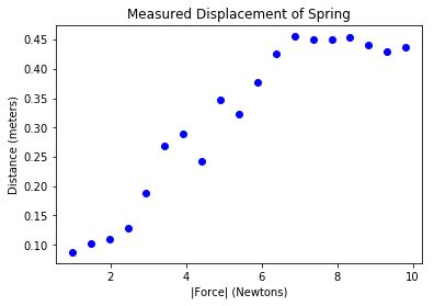
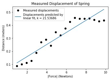
图18-5 使用曲线拟合数据
In [7]: def fitData(inputFile):
   ...:     masses, distances = getData(inputFile)
   ...:     distances = pylab.array(distances)
   ...:     forces = pylab.array(masses)*9.81
   ...:     pylab.plot(forces, distances, 'ko',
   ...:         label = 'Measured displacements')
   ...:     pylab.title('Measured Displacement of Spring')
   ...:     pylab.xlabel('|Force| (Newtons)')
   ...:     pylab.ylabel('Distance (meters)')
   ...:     #find linear fit
   ...:     a,b = pylab.polyfit(forces, distances, 1)
   ...:     predictedDistances = a*pylab.array(forces) + b
   ...:     k = 1.0/a #see explanation in text
   ...:     pylab.plot(forces, predictedDistances,
   ...:         label = 'Displacements predicted by\nlinear fit, k = '
   ...:             + str(round(k, 5)))
   ...:     pylab.legend(loc = 'best')
   ...:

In [8]: fitData('springData.txt')
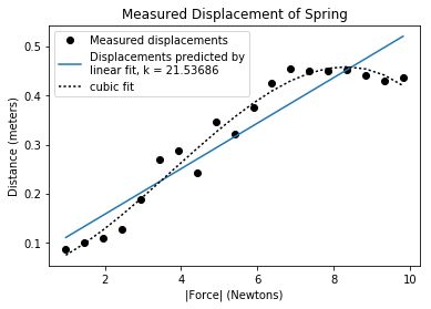
我们向fitData添加一些代码,试一下三次拟合。
注意直接在原来的代码下面进行追加是不行的,要注意添加到代码再源代码
#find cubic fit
fit = pylab.polyfit(forces, distances, 3)
predictedDistances = pylab.polyval(fit, forces)
pylab.plot(forces, predictedDistances, 'k:', label = 'cubic fit')
In [15]: def fitData(inputFile):
    ...:    masses, distances = getData(inputFile)
    ...:    distances = pylab.array(distances)
    ...:    forces = pylab.array(masses)*9.81
    ...:    pylab.plot(forces, distances, 'ko',
    ...:        label = 'Measured displacements')
    ...:    pylab.title('Measured Displacement of Spring')
    ...:    pylab.xlabel('|Force| (Newtons)')
    ...:    pylab.ylabel('Distance (meters)')
    ...:    #find linear fit
    ...:    a,b = pylab.polyfit(forces, distances, 1)
    ...:    fit = pylab.polyfit(forces, distances, 3) ## 1
    ...:    predictedDistances = a*pylab.array(forces) + b
    ...:    k = 1.0/a #see explanation in text
    ...:    pylab.plot(forces, predictedDistances,
    ...:        label = 'Displacements predicted by\nlinear fit, k = '
    ...:            + str(round(k, 5)))
    ...:    predictedDistances = pylab.polyval(fit, forces) ## 2
    ...:    pylab.plot(forces, predictedDistances, 'k:', label = 'cubic fit')
    ...:    pylab.legend(loc = 'best')
    ...:

In [16]: fitData('springData.txt')
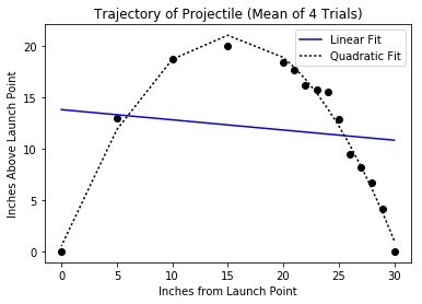
弹丸的行为:
In [9]: def getTrajectoryData(fileName):
   ...:     dataFile = open(fileName, 'r')
   ...:     distances = []
   ...:     heights1, heights2, heights3, heights4 = [],[],[],[]
   ...:     dataFile.readline()
   ...:     for line in dataFile:
   ...:         d, h1, h2, h3, h4 = line.split()
   ...:         distances.append(float(d))
   ...:         heights1.append(float(h1))
   ...:         heights2.append(float(h2))
   ...:         heights3.append(float(h3))
   ...:         heights4.append(float(h4))
   ...:     dataFile.close()
   ...:     return (distances, [heights1, heights2, heights3, heights4])
   ...:

In [10]: def processTrajectories(fileName):
    ...:    distances, heights = getTrajectoryData(fileName)
    ...:    numTrials = len(heights)
    ...:    distances = pylab.array(distances)
    ...:    #生成一个数组,用于存储每个距离的平均高度
    ...:    totHeights = pylab.array([0]*len(distances))
    ...:    for h in heights:
    ...:        totHeights = totHeights + pylab.array(h)
    ...:    meanHeights = totHeights/len(heights)
    ...:    pylab.title('Trajectory of Projectile (Mean of '\
    ...:            + str(numTrials) + ' Trials)')
    ...:    pylab.xlabel('Inches from Launch Point')
    ...:    pylab.ylabel('Inches Above Launch Point')
    ...:    pylab.plot(distances, meanHeights, 'ko')
    ...:    fit = pylab.polyfit(distances, meanHeights, 1)
    ...:    altitudes = pylab.polyval(fit, distances)
    ...:    pylab.plot(distances, altitudes, 'b', label = 'Linear Fit')
    ...:    fit = pylab.polyfit(distances, meanHeights, 2)
    ...:    altitudes = pylab.polyval(fit, distances)
    ...:    pylab.plot(distances, altitudes, 'k:', label = 'Quadratic Fit')
    ...:    pylab.legend()
    ...:

In [11]: processTrajectories('launcherData.txt')
19章 随机试验与假设检验
在统计学中,显著性检验是“统计假设检验”(Statistical hypothesis testing)的一种,显著性检验是用于检测科学实验中实验组与对照组之间是否有差异以及差异是否显著的办法。“统计假设检验”这一正名实际上指出了“显著性检验”的前提条件是“统计假设”,换言之“无假设,不检验”。用更通俗的话来说就是要先对科研数据做一个假设,然后用检验来检查假设对不对。一般而言,把要检验的假设称之为原假设,记为H0;把与H0相对应(相反)的假设称之为备择假设,记为H1。
如果原假设为真,而检验的结论却劝你放弃原假设。此时,我们把这种错误称之为第一类错误。通常把第一类错误出现的概率记为α 如果原假设不真,而检验的结论却劝你不放弃原假设。此时,我们把这种错误称之为第二类错误。通常把第二类错误出现的概率记为β
通常只限定犯第一类错误的最大概率α, 不考虑犯第二类错误的概率β。我们把这样的假设检验称为显著性检验,概率α称为显著性水平。显著性水平是数学界约定俗成的,一般有α =0.05,0.025.0.01这三种情况。代表着显著性检验的结论错误率必须低于5%或2.5%或1%(统计学中,通常把在现实世界中发生几率小于5%的事件称之为“不可能事件”)。
In [18]: import scipy

In [19]: tStat = -2.13165598142 #t-statistic for PED-X example
    ...: tDist = []
    ...: numBins = 1000
    ...: for i in range(10000000):
    ...:    tDist.append(scipy.random.standard_t(198))
    ...:
    ...: pylab.hist(tDist, bins = numBins,
    ...:        weights = pylab.array(len(tDist)*[1.0])/len(tDist))
    ...: pylab.axvline(tStat, color = 'w')
    ...: pylab.axvline(-tStat, color = 'w')
    ...: pylab.title('T-distribution with 198 Degrees of Freedom')
    ...: pylab.xlabel('T-statistic')
    ...: pylab.ylabel('Probability')
    ...:
Out[19]:

是否显著

In [21]: import random

林赛的游戏模拟
In [22]: numGames = 1273
    ...: lyndsayWins = 666
    ...: numTrials = 10000
    ...: atLeast = 0
    ...: for t in range(numTrials):
    ...:    LWins = 0
    ...:    for g in range(numGames):
    ...:        if random.random() < 0.5:
    ...:            LWins += 1
    ...:    if LWins >= lyndsayWins:
    ...:        atLeast += 1
    ...: print('Probability of result at least this',
    ...: 'extreme by accident =', atLeast/numTrials)
    ...:
Probability of result at least this extreme by accident = 0.0479

正确的游戏模拟
In [23]: numGames = 1273
    ...: lyndsayWins = 666
    ...: numTrials = 10000
    ...: atLeast = 0
    ...: for t in range(numTrials):
    ...:    LWins, JWins = 0, 0
    ...:    for g in range(numGames):
    ...:        if random.random() < 0.5:
    ...:            LWins += 1
    ...:        else:
    ...:            JWins += 1
    ...:    if LWins >= lyndsayWins or JWins >= lyndsayWins:
    ...:        atLeast += 1
    ...: print('Probability of result at least this',
    ...: 'extreme by accident =', atLeast/numTrials)
    ...:
Probability of result at least this extreme by accident = 0.1054
p值
P 值就是当原假设为真时所得到的样本观察结果或更极端结果出现的概率。如果 P 值很小,说明这种情况的发生的概率很小,而如果出现了,根据小概率原理,我们就有理由拒绝原假设,P 值越小,我们拒绝原假设的理由越充分。
总之,P 值越小,表明结果越显著。但是检验的结果究竟是 “显著的”、“中度显著的” 还是 “高度显著的” 需要我们自己根据 P 值的大小和实际问题来解决。
20章 条件概率和贝叶斯定理,参见《统计学习方法》
李航-第4章朴素贝叶斯法
参考链接:
关于显著性检验,你想要的都在这儿了!!(基础篇)
不得不提的 P 值
显著性水平 P值 概念解释