点击这里进入人工智能嘚吧嘚目录,观看全部文章
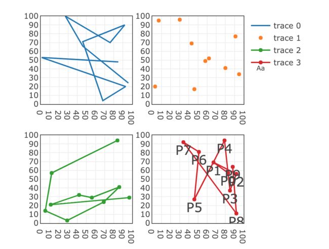
Scatter散点图和子图subplots
各种scatter的mode,以FigureWidget为容器的子图表。
注意这里的为layout使用了'xaxis1','xaxis2'...’yaxis1','yaxis2'...来为每个图表应用布局。
from plotly import tools
import plotly.offline as py
import plotly.graph_objs as go
import random
py.init_notebook_mode()

axis_style = dict(
    autorange=False,
    range=(0, 100),
    dtick=10,
    showline=True,
    mirror='ticks',
)
layout = go.Layout(autosize=False, width=500, height=500)

modes = ["lines", "markers", "lines+markers", "lines+markers+text"]

subplot = tools.make_subplots(2, 2, print_grid=False)
fig = go.FigureWidget(subplot)

for n in range(len(modes)):
    data = go.Scatter(
        x=[random.randint(0, 100) for n in range(10)],
        y=[random.randint(0, 100) for n in range(10)],
        text=['P{}'.format(t) for t in range(10)],
        textposition='bottom center',
        textfont={'size': 20},
        mode=modes[n])
    layout['xaxis{}'.format(n + 1)] = axis_style
    layout['yaxis{}'.format(n + 1)] = axis_style
    fig.add_trace(data, row=int(n / 2) + 1, col=n % 2 + 1)
fig['layout'].update(layout)
py.iplot(fig)
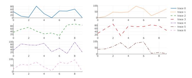
折线图和子图
下面的subplots没有使用FigureWidget,也没有为每个子图定制layout。
下面代码也展示了各种虚线类型的使用方法。
from plotly import tools
import plotly.offline as py
import plotly.graph_objs as go
import random
py.init_notebook_mode()

dashes = ["solid", "dot", "dash", "longdash", "dashdot", "longdashdot","5px,10px,2px,2px"]

fig = tools.make_subplots(rows=4, cols=2)

for n in range(len(dashes)):
    data = go.Scatter(
        x=[n for n in range(10)],
        y=[random.randint(0, 100) for n in range(10)],
        text=['P{}'.format(t) for t in range(10)],
        textposition='bottom center',
        textfont={'size': 20},
        mode='lines',
        line = {'dash':dashes[n]}
    )
    fig.add_trace(data, row=int(n / 2) + 1, col=n % 2 + 1)

py.iplot(fig)
三维图和子图
注意make_subplots方法的specs参数要与row和col对齐,横行竖行的每个图都要设定{ 'is_3d': True}。
from plotly import tools
import plotly.offline as py
import plotly.graph_objs as go
import random
py.init_notebook_mode()

subplot3d1 = go.Scatter3d(
    x=[random.random() for n in range(100)],
    y=[random.random() for n in range(100)],
    z=[random.random()*10 for n in range(100)],
    mode='markers',
    marker=dict(size=8, color=z, colorscale='Viridis',opacity=0.5))

subplot3d2 = go.Surface(
    z=[[(x * x + y * y) for x in range(-100, 100)] for y in range(-100, 100)],
    opacity=1)

fig = tools.make_subplots(
    rows=1, cols=2, specs=[[{
        'is_3d': True
    }, {
        'is_3d': True
    }]])
fig.append_trace(subplot3d1, 1, 1)
fig.append_trace(subplot3d2, 1, 2)

py.iplot(fig)

更多请参考官方文档:
3d-scatter-plots
3d-surface-plots
reference
3d-subplots
subplots
点击这里进入人工智能DBD嘚吧嘚目录,观看全部文章
每个人的智能新时代
如果您发现文章错误,请不吝留言指正;
如果您觉得有用,请点喜欢;
如果您觉得很有用,欢迎转载~
END