predict函数 R_R语言机器学习:mlr包的使用和模型解释(连续变量)
作者:黄天元,复旦大学博士在读,热爱数据科学与开源工具(R),致力于利用数据科学迅速积累行业经验优势和学术知识发现。知乎专栏:R语言数据挖掘 邮箱:[email protected].欢迎合作交流。
R语言中,能够构建统一的机器学习框架的包除了caret之外,还有一个更加精细的包叫做mlr。比起caret,它能够设置的参数更加多,能够定制更加细致的框架。但是也是因为如此,与caret相比它要难上手一些,因为必须要懂得更多参数的内在含义才能够正确有效地使用它。本文参考
# 1 载入包和数据
```{r}
library(DALEX)
library(mlr)
library(breakDown)
data(apartments)
head(apartments)
```
# 2 建模与分析
这里要讲关于mlr包建模的一些细节。首先,需要定义任务,也就是告诉模型我们需要做的是分类问题还是回归问题。需要使用makeRegrTask函数对其定义,其中id参数给这个任务做命名,data测存放数据,target参数用来告诉函数哪个变量是响应变量。具体代码如下:
```{r}
set.seed(123)
regr_task <- makeRegrTask(id = "ap", data = apartments, target = "m2.price")
```
其次,我们需要对模型进行定义。这里采用随机森林、神经网络和广义增强模型建模(GBM模型,本质还是基于树的ensemble,具体看这个gbm包的介绍)。
```{r}
regr_lrn_rf <- makeLearner("regr.randomForest")
regr_lrn_nn <- makeLearner("regr.nnet")
regr_lrn_gbm <- makeLearner("regr.gbm", par.vals = list(n.trees = 500))
```
对于神经网络而言,需要对超参数进行额外的调整(多少隐藏层、迭代次数),而且需要对数据进行预处理(中心化标准化)。
```{r}
regr_lrn_nn <- setHyperPars(regr_lrn_nn, par.vals = list(maxit=500, size=2))
regr_lrn_nn <- makePreprocWrapperCaret(regr_lrn_nn, ppc.scale=TRUE, ppc.center=TRUE)
```
随后要进行的是模型的训练,任务和模型定义好之后,可以快速训练。
```{r}
regr_rf <- train(regr_lrn_rf, regr_task)
regr_nn <- train(regr_lrn_nn, regr_task)
regr_gbm <- train(regr_lrn_gbm, regr_task)
```
接下来,要定义预测函数。也就是如果我们给一个测试集,那么模型怎么样才能够得到想要的预测值。
```{r}
data(apartmentsTest)
custom_predict <- function(object, newdata) {pred <- predict(object, newdata=newdata)
response <- pred$data$response
return(response)}
explainer_regr_rf <- DALEX::explain(regr_rf, data=apartmentsTest, y=apartmentsTest$m2.price, predict_function = custom_predict, label="rf")
explainer_regr_nn <- DALEX::explain(regr_nn, data=apartmentsTest, y=apartmentsTest$m2.price,
predict_function = custom_predict, label="nn")
explainer_regr_gbm <- DALEX::explain(regr_gbm, data=apartmentsTest, y=apartmentsTest$m2.price,
predict_function = custom_predict, label="gbm")
```
一般而言,函数的设计需要在第一个参数object中放入一个模型,而newdata代表测试数据集,最后返回的是利用这个模型和测试数据集的解释变量所计算得到的预测数值。
后面就是模型解释的常规套路了,这里不再赘述,感兴趣的可以看之前的帖子(
# 3 常规模型解释套路代码搬运

```{r}
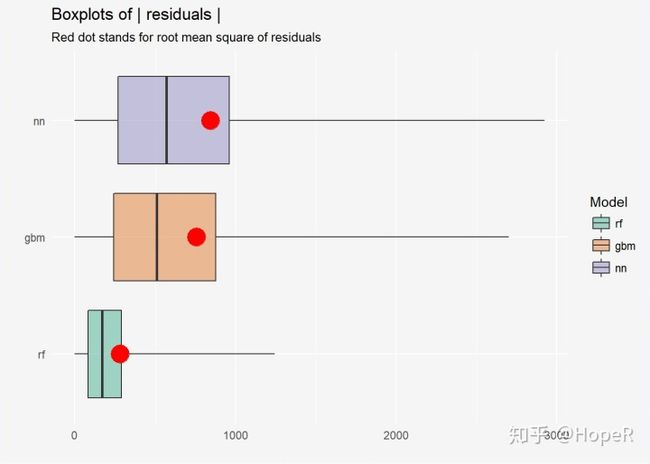
##模型表现分析
mp_regr_rf <- model_performance(explainer_regr_rf)
mp_regr_gbm <- model_performance(explainer_regr_gbm)
mp_regr_nn <- model_performance(explainer_regr_nn)
mp_regr_rf
plot(mp_regr_rf, mp_regr_nn, mp_regr_gbm)
plot(mp_regr_rf, mp_regr_nn, mp_regr_gbm, geom = "boxplot")
##变量重要性分析
vi_regr_rf <- variable_importance(explainer_regr_rf, loss_function = loss_root_mean_square)
vi_regr_gbm <- variable_importance(explainer_regr_gbm, loss_function = loss_root_mean_square)
vi_regr_nn <- variable_importance(explainer_regr_nn, loss_function = loss_root_mean_square)
plot(vi_regr_rf, vi_regr_gbm, vi_regr_nn)
```

不过,这里介绍一个新的参数设置,就是`type = "difference"`。在求变量重要性的时候,默认给出的是如果失去了这个变量,那么模型会发生的实质数值变化。如果把这个参数设置为`ratio`,那么就是缺失这个变量与缺失所有变量的变化之比,而设置为`difference`则为变化之差。这些参数能够让我们使用更加丰富的手段判断一个变量的重要程度。
```{r}
vi_regr_rf <- variable_importance(explainer_regr_rf, loss_function = loss_root_mean_square, type="difference")
vi_regr_gbm <- variable_importance(explainer_regr_gbm, loss_function = loss_root_mean_square, type="difference")
vi_regr_nn <- variable_importance(explainer_regr_nn, loss_function = loss_root_mean_square, type="difference")
plot(vi_regr_rf, vi_regr_gbm, vi_regr_nn)
```

下面做常规的单变量探索图:
```{r}
## PDP图
pdp_regr_rf <- variable_response(explainer_regr_rf, variable = "construction.year", type = "pdp")
pdp_regr_gbm <- variable_response(explainer_regr_gbm, variable = "construction.year", type = "pdp")
pdp_regr_nn <- variable_response(explainer_regr_nn, variable = "construction.year", type = "pdp")
plot(pdp_regr_rf, pdp_regr_gbm, pdp_regr_nn)
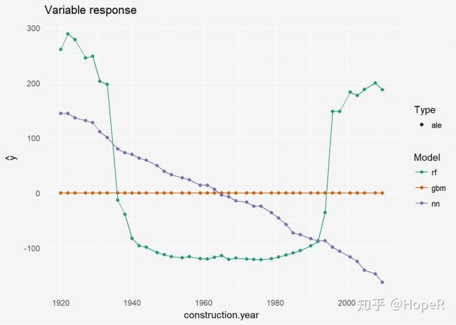
## ALE图
ale_regr_rf <- variable_response(explainer_regr_rf, variable = "construction.year", type = "ale")
ale_regr_gbm <- variable_response(explainer_regr_gbm, variable = "construction.year", type = "ale")
ale_regr_nn <- variable_response(explainer_regr_nn, variable = "construction.year", type = "ale")
plot(ale_regr_rf, ale_regr_gbm, ale_regr_nn)
```

最后是对因子变量的探索:
```{r}
mpp_regr_rf <- variable_response(explainer_regr_rf, variable = "district", type = "factor")
mpp_regr_gbm <- variable_response(explainer_regr_gbm, variable = "district", type = "factor")
mpp_regr_nn <- variable_response(explainer_regr_nn, variable = "district", type = "factor")
plot(mpp_regr_rf, mpp_regr_gbm, mpp_regr_nn)
```
