深度学习之---卷积神经网络

1.简介

本篇介绍卷积神经网络。今年来深度学习在计算机视觉领域取得突破性成果的基石。目前的工业场景应用也是越来越多，比如自然语言处理、推荐系统和语音识别等领域广泛使用。下面会主要描述卷积神经网络中卷积层和池化层的工作原理，并解释填充、步幅、输入通道和输出通道的含义。
后面也会介绍一点比较有代表性的神经网络网络结构，比如：AlexNet、VGG、NiN、GoogLeNet、ResNet、DenseNet。

2.二维卷积层

什么是二维卷积层？

• 卷积神经网络(convolutional neural network)是含有卷积层(convlutional layer)的神经网络。
• 所谓二维卷积层，就是只有两个维度的卷积神经网络，只有高和宽两个空间维度，常用来处理图像数据。

【二维互相关运算】

• 虽然卷积层得名于卷积运算，但我们通常在卷积层中使用更加直观的互相关运算。
• 在二维卷积中，一个二维输入数组和一个二维核数组通过互相关运算输出一个二维数组。
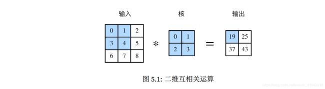
• 如下图的二维互相关运算，输入是一个高和宽都是3的二维数组；核是一个2 x 2 的二维数组。
• 核，又称作卷积核或过滤器。卷积核窗口的形状取决于卷积核的高贺宽，即2 x 2 。
• 那怎么计算：0 × 0 + 1 × 1 + 3 × 2 + 4 × 3 = 19。简单描述就是，对应位置元素相乘再相加。
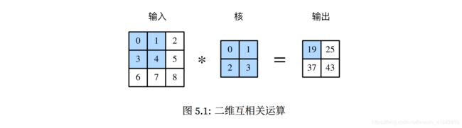
• 整个运算，卷积窗口从输入数组的最上方开始，从左到右、从上到下，依次在输入数组上滑动。每滑动一次就计算一次。

【二维卷积层】

• 二维卷积层将输入和卷积核做互相关运算，并加上一个标量偏差来得到输出。卷积层的模型参数包括了卷积核和标量偏差。在训练模型的时候，通常我们对卷积核随机初始化，然后不断迭代卷积核和偏差。

【图像中物体边缘检测】

• 检测图像中物体的边缘，也就是找到像素变化的位置。
• 举个栗子：构造一个6 x 8图片。中间4列为黑色，其余为白色。目标是寻找到黑色和白色的边界。
  
• 用一个1 x 2 的卷积核进行卷积操作。
  
• 进行完成二维互相关运算后得出结果。
  
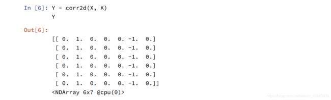
• 由栗子可以看到，卷积层可以通过重复使用卷积核有效的表征局部空间。

【互相关运算和卷积运算】

• 实际上，卷积运算和互相关运算类似。
• 为了得到卷积运算的输出，我们只需要将核数组左右翻转并上下翻转，再与输入数组做互相关运算。
• 可见，卷积运算和互相关运算虽然类似，但如果它们使用相同的核数组，对于同一个输入，输出往往并不相同。
• 那么，肯定会有同学好奇，卷积层为何能使用互相关运算替代卷积运算。
• 其实，在深度学习中核数组都是学出来的：卷积层无论使用互相关运算或者卷积运算都不影响模型预测时的输出。
• 为了解释这一点，假设卷积层使用互相关运算学出图5.1中的核数组，设其他条件不变，使用卷积运算学出的核数组，即图5.1中的核数组按上下、左右翻转。也就是说。图5.1中的输入与学出的已翻转的核数组再做卷积运算时，依然得到图5.1中的输出。

【特征图和感受野】

• 二维卷积层输出的二维数组可以看做是输入在空间维度（宽和高）上某一级的表征，也叫做特征图(feature map)。影响元素$x$的前向计算的所有可能输入区域（可能大于输入的实际尺寸）叫做$x$的感受野(receptive field)。
• 以图5.1为例，输入中阴影部分的四个元素是输出中阴影部分元素的感受野。

• 将图5.1中形状为2 x 2 的输出记为$Y$，并考虑一个更深的卷积神经网络：将$Y$与另一个形状为2 x 2 的核数组做互相关运算，输出单个元素$z$。
• 那么，$z$在$Y$上的感受野包括$Y$的全部四个元素，在输入上的感受野包括其中全部9个元素。
• 可见，可以通过更深的卷积神经网络使得特征图中单个元素的感受野变得更加广阔，从而捕捉输入上更大尺寸的特征。
• 这里所说的“元素”，描述的是矩阵中的成员。有的地方也称作“单元”。

3.填充和步幅

上面提到了卷积运算，我们知道，使用3 x 3 的输入，与2 x 2 的卷积核得到的输出是 2 x 2 ；一般来说，假设输入的形状是$n_h\ast n_w$，卷积核窗口形状是$k_h\ast k_w$，那么输出形状将会是：
$$(n_h-k_h+1)\ast (n_w-k_w+1).$$
所以，卷积层的输出形状有输入形状和卷积核窗口形状决定。下面介绍的卷积层的两个超参数，即填充和步幅。它们可以对给定形状的输入和卷积核改变输出形状。

【填充】

• 填充（padding）是指在输入高和宽的两侧填充元素(通常是0元素)。
• 如下图，就是对原来的图像进行了padding处理

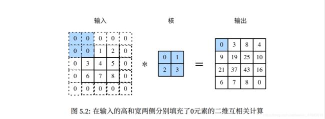
• 一般来说，如果在高的两侧一共填充$p_h$行，在宽的两侧一共填充$p_w$列，那么输出形状将会是：
  $$(n_h-k_h+p_h+1)\ast (n_w-k_w+p_w+1).$$
• 也就是说，输出的高和宽会分别增加$p_h$和$p_w$.
• 很多情况下，我们会设置$p_h=k_h-1$和$p_w=k_w-1$来使得输入和输出具有相同的高和宽。这样会方便在构造网络时推测每个层的输出形状。
• 假设这里的$k_h$是奇数，我们会在高的两侧分别填充$p_h/2$行。如果$k_h$是偶数，一种可能是在输入的顶端一侧填充$p_h/2$行，而在底端一侧填充$p_h/2$行。在宽的两侧填充同理。
• 卷积神经网络经常使用奇数高宽的卷积核，如1、3、5和7，所以两端上的填充个数相等。对任意的二维数组X，设它的第$i$行,第$j$列的元素为X[i,j]。当两端上的填充个数相等，并使输入输出具有相同的高和宽时，我们就知道输出Y[i,j]是由输入以X[i,j]为中心的窗口同卷积核进行互相关计算得到的。

【步幅】

• 上面提到的二维互相关运算。卷积窗口从输入数组的最左上方开始，从左到右，从上到下，依次在输入数组上滑动。我们将每次滑动的行数和列数称为步幅(stride)
• 前面的例子里，在高和宽两个方向上步幅都为1
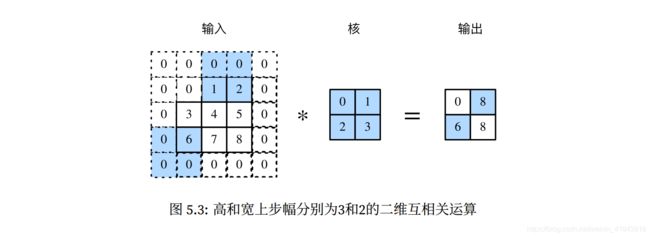
• 在下图的栗子里，步幅就比较大一些，在高上步幅为3，在款上步幅为2.
• 可以看到，在宽方向上滑动时，由于输入无法填满窗口，无结果输出。
  
• 一般来说，当高上步幅为$s_h$，宽上步幅为$s_w$时，输出形状为：
  $$[(n_h-k_h+p_h+s_h)/s_h]\ast [(n_w-k_w+p_w+s_w)/s_w].$$
• 如果设置$p_h=k_n-1$和$p_w=k_w-1$，那么输出形状可以简化为：
  $$[(n_h+s_h-1)/s_h]\ast [(n_w+s_w-1)/s_w].$$
• 更进一步，如果输入的高和宽能分别被高和宽上的步幅整除，那么输出的形状将是：
  $$[n_h/s_h]\ast [n_w/s_w].$$
• 填充可以增加输出的高和宽，这常用来使得输出与输入具有相同的高和宽。
• 步幅可以减小输出的高和宽。

4.多输入和多输出通道

上面所说的输入和输出都是二维的数组，但真实数据的维度经常更高。例如，彩色图像在高和宽2个维度外还有RGB（红、绿、蓝）3个颜色通道，假设彩色图像的高和宽分别为h和w（像素），那么它可以表示为一个3hw的多维数组。我们将大小为3的这一维称为通道（channel）维。下面就介绍含多个输入通道或多个输出通道的卷积核。

【多输入通道】

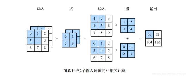
• 当输入数据含有多个通道时，我们需要构造一个输入通道数与输入数据的通道数相同的 卷积核，从而能够与含有多个通道的输入做互相关运算。
• 假如输入数据的通道数为3个，那么卷积核的输入的通道数同样为3个。
• 假设卷积核的窗口形状为2 x 2 ，有3个输入通道，那么就会有3个卷积核，将这3个输入通道连接起来，就会形成一个形状为 3 x 2 x 2 的卷积核。
• 下面是一个含有2个输入通道的互相关运算。

【多输出通道】

• 当输入通道有多个时，因为我们对各个通道的结果做了累加，所以不论输入通道数是多少，输出通道数总是为1.
• 设卷积输入通道数和输出通道数分别为$c_i和c_o$，高和宽分别为$k_h和k_w$。如果希望得到含有多个通道的输出，我们可以为每个输出通道分别为创建形状为$c_i\ast k_h\ast k_w$的核数组。将他们在输出通道上连接。卷积核的形状即为$c_o\ast c_i\ast k_h\ast k_w$。在做互相关运算是，每个输出通道上的结果由卷积核在该输出通道上的核数组数与整个输入数组计算而来。

【卷积层】

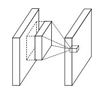
• 最后讨论卷积窗口为1 x 1的多通道卷积层。通常，称之为1 x 1卷积层，并将其中的卷积运算称为1 x 1 卷积。
• 因为使用了最小的窗口，1 x 1卷积失去了卷积层可以识别高和宽维度上相邻元素构成的模式的功能。
• 实际上，1 x 1卷积的主要计算发生在通道维上。
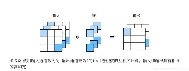
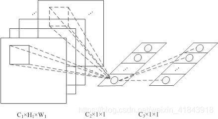
• 下图展示了使用输入通道数为3、输出通道数为2的1 x 1卷积核的互相关运算，要注意，输入和输出具有相同的高和宽。输出中的每个元素来自输入中在高和宽上相同位置的元素，在不同同通道之间的按权重累加。
• 假设我们将通道维当做特征维度，将高和宽维度上的元素当成数据样本，那么1 x 1卷积层的作用与全连接层等价。

• 在后面的模型里我们会看到1 x 1 的卷积层被当做保持高和宽维度形状不变的全连接层使用。于是，我们可以通过调整网络层之间的通道数来控制模型复杂度。
• 使用多通道可以拓宽卷积层的模型参数。
• 假设将通道维当作特征维，将高和宽维度上的元素当成数据样本，那么1 x 1 卷积层的作用与全连接层等价。
• 1 x 1卷积层通常用来调整网络层之间的通道数，并控制模型复杂度。

5.池化层

在“二维卷积层”中，有说过图像物体边缘检测的应用，我们构造卷积核从而精确找到了像素变化的位置。

• 设任意⼆维数组X的i⾏j列的元素为$X[i,j]$。如果我们构造的卷积核输出Y[i, j]=1，那么说明输⼊中$X[i,j]$和$X[i,j+1]$数值不⼀样。这可能意味着物体边缘通过这两个元素之间。
• 但实际图像里，我们感兴趣的物体不会总出现在固定位置：即使我们连续拍摄同一个物体也极有可能出现像素位置上的偏移。这会导致同一个边缘对应的输出可能出现在卷积输出$Y$中的位置不同，进而对后面的模式识别造成不便。
• 下面介绍的池化层，它的提出是为了缓解卷积层对位置的过度敏感性。

【二维最大池化层和平均池化层】

• 同卷积层的滑动方式一样，池化层每次对输入数据的一个固定形状窗口（又称为池化窗口）中的元素计算输出。
• 不同于卷积层里计算和核的互相关性，池化层直接计算池化窗口内元素的最大值或者平均值。
• 该运算也分别叫做最大化池化或平均池化。
• 在二维最大池化中，池化窗口从输入数组的最左上方开始，按从左往右、从上往下的顺序，依次在输入数组上滑动。当池化窗口滑动到某一位置时，窗口中的输入子数组的最大值即输出数组中相应位置的元素。

• 上图展示了池化窗口形状为2 x 2的最大池化。
• 相对的计算平均池化，原理与最大池化类似，但是将最大运算符替换成平均运算符。
• 让我们再次回到本节开始提到的物体边缘检测的例⼦。现在我们将卷积层的输出作为2 × 2最⼤池化的输⼊。设该卷积层输⼊是X、池化层输出为Y。⽆论是$X[i,j]$和$X[i,j+1]$值不同，还是$X[i,j+1]$和$X[i,j+2]$不同，池化层输出均有$Y[i,j]=1$。也就是说，使⽤2 × 2最⼤池化层时，只要卷积层识别的模式在⾼和宽上移动不超过⼀个元素，我们依然可以将它检测出来。

【填充和步幅】

• 同卷积层一样，池化层也可以在输入的高和宽两侧的填充并调整窗口的移动步幅来改变输出形状。
• 池化层填充和步幅与卷积层填充和步幅的工作机制一样。

【多通道】

• 在处理多通道输入数据时，池化层对每个输入通道分别池化，而不是像卷积层那样将各个通道的输入按通道相加。
• 这意味着池化层的输出通道数与输入通道数是相同的。

【概括】

• 最大池化和平均池化分别取池化窗口中输入元素的最大值和平均值作为输出。
• 池化层的一个主要作用是缓解卷积层对位置的过度敏感性。
• 可以指定池化层的填充和步幅。
• 池化层的输出通道数跟输入通道数相同。

6.卷积神经网络（LeNet）

在前面使用的，一个含有单隐层的多层感知机模型对MNIST数据集中的图像进行分类。每张图像高和宽均是28像素。将每个图像进行展开，得到长度为784的向量，并输入进全连接层。然而，这种分类方法有一定的局限性。

• 1.图像在同一列邻近的像素在这个向量中可能相距较远。它们构成的模式可能难以被模型识别。
• 2.对于大尺寸的输入图像，使用全连接层容易造成模型过大。假设输入是高和宽均为1000像素的彩色照片（含有3个通道）。即使全连接层输出个数仍然是256个，该层的权重参数的形状为3000000 x 256，它占用了大约3GB的内存或者显存。这带来过复杂的模型和过高的存储开销。

卷积层尝试决绝这两个问题：

• 一方面，卷积层保留输入形状，使得图像的像素在高和宽两个方向上的相关性均可能被有效识别
• 另一方面，卷积层通过滑动窗口将同一卷积核与不同位置的输入重复计算，从而避免参数过大。

卷积神经网络就是含有卷积层的网络。LeNet可以说是神经网络的开山鼻祖，在这个网络中包含了前面提到的卷积层、池化层、激活层、全连接层，该网络结构最早被应用于手写数字图像识别，作者叫Yann LeCun，这也是LeNet名字的由来；LeNet展示了通过梯度下降训练卷积神经网络可以达到手写数字识别在当时最先进的结果，这个奠基性的工作第一次将卷积神经网络推上舞台，为众人所知。

【LeNet模型】

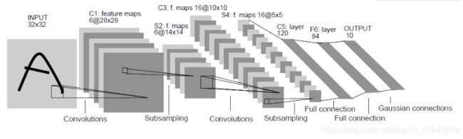
• LeNet分为卷积层块和全连接层块两个部分：

  • 卷积层块里的基本单位是卷积层后接最大池化层。
    • 卷积层用来识别图像里的空间模式，如线条和物体的局部。
    • 最大池化层用来降低卷积层对位置的敏感性。
    • 卷积层由这两个这样的基本单位重复堆叠构成。
    • 在卷积层块中，每个卷积层都使用5 x 5的窗口，并输出上使用ReLU激活函数。
    • 卷积层的详细信息下面介绍。
  • 全联机层块输入形状将变成二维。

• 这是最最原始的LeNet网络结构，目前来说已经成为历史，我们看后面的改进版本
  

• 这是改进后的LeNet-5版本，在原来的基础上进行了一些优化调整。

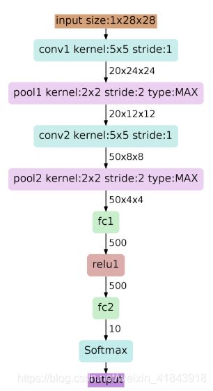
• 下面对上面的网络架构进行解释：
  • 1.输入图像是单通道的28 x 28 大小的图像，用矩阵表示[1,28,28]。
  • 2.第一个卷积层conv1，卷积核为5 x 5，通道数为20，步长1，经过卷积后，图像尺寸变为28 - 5 + 1 = 24，用矩阵表示[20,24,24]。
  • 3.第一个池化层Max1，最大化池化，池化核尺寸为2 x 2，步长为2，无重叠池化，经过池化后，图像尺寸减半，变为12，用矩阵表示[20,12,12]。
  • 4.第二个卷积层conv2，卷积核为5 x 5，通道数为50，步长1，经过卷积后，图像尺寸变为12 - 5 + 1 = 8，用矩阵表示[50,8,8]。
  • 5.第二个池化层Max2，最大化池化，池化核尺寸为2 x 2，步长为2，无重叠池化，经过池化后，图像尺寸减半，变为4，用矩阵表示[50,4,4]。
  • 6.第一个全连接层fc1，神经元个数为500个，得到一个500维的向量特征。后面作用一个ReLu的激活函数.
  • 7.第二个全连接层fc2，神经元个数为10个，得到一个10维的向量特征。后面作用一个softmax函数，用于预测手写体数字的10个分类的预测。
• 下面给出基于Keras的一个实现

def LeNet():
	# 定义模型
    model = Sequential()
    # conv1
    model.add(Conv2D(32,(5,5),strides=(1,1),input_shape=(28,28,1),padding='valid',activation='relu',kernel_initializer='uniform'))
    # max1
    model.add(MaxPooling2D(pool_size=(2,2)))
    # conv2
    model.add(Conv2D(64,(5,5),strides=(1,1),padding='valid',activation='relu',kernel_initializer='uniform'))
    # max2
    model.add(MaxPooling2D(pool_size=(2,2)))
    # 多通道压平
    model.add(Flatten())
    # fc1
    model.add(Dense(500,activation='relu'))
    # fc2
    model.add(Dense(10,activation='softmax'))
    return model

【概括】

• 卷积神经网络就是含有卷积层的网络
• LeNet交替使用卷积层和最大池化层后接全连接层来进行图像分类。

7.深度卷积神经网络（AlexNet）

在LeNet提出后的将近20年里，神经网络一度被其他机器学习方法超越，如SVM。虽然LeNet可以在早期的小数据集上取得好的成绩，但是在更大的真实数据集上的表现并不是很令人满意。

• 一方面，神经网络计算复杂。在没有GPU的加持下，计算力不足。
• 另一方面，当年的研究者还没有大量深入研究参数初始化和非凸优化算法等诸多领域。

在上面的LeNet中看到，神经网络可以直接基于图像分类的原始像素进行分类，这种称为端到端(end - to - end)的方法节省了很多中间步骤。然而，在很长一段时间里更流行的是研究者通过勤劳与智慧所涉及并生成的手动特征，这类图像分类研究的主要流程是：

• 1.获取图像数据集
• 2.使用已有的特征提取函数生产图像的特征
• 3.使用机器学习模型对图像的特征分类。

当时认为的机器学习部分仅限最后这一步，如果那时候跟机器学习研究者交谈，他们认为机器学习既重要又优美。优美的定理证明了许多分类器的性质。机器学习领域生机勃勃、严谨而且机器有用。然而，如果跟计算机视觉研究者交谈，则是另外一幅景象。他们会告诉你图像识别里“不可告人”的现实是：计算机视觉流程中真正重要的是数据和特征。也就是说，使用较干净的数据和较有效的特征甚至比机器学习模型的选择对图像分类结果的影响更大。

【学习特征表示】
特征如此的重要，如何去表征他就成为了一个很关键的问题。
在上面的学习中，特征的提取方式有两种：

• 1.基于各式各样手工设计的函数从数据中提取。
• 2.特征的本身应该由学习得来，并且为了表征足够复杂的输入，特征本身应该分级表示。
  • 在上面的“二维卷积层”的部分，这种分级表示其实已经初现端倪。
  • 图像第一级的表示可以是特定的位置和角度是否出现边缘。
  • 图像第二级的表示可以是这些边缘组合的其他模式，比如花纹。
  • 图像第三季的表示可以是上一级花纹的更一步融合，得到对应物体特定部位的模式。
  • 如此逐级表示下去。最终，模型能够较容易根据最后一级的表示完成分类任务
  • 需要注意的是：输入的逐级表示由多层模型中测参数确定，而这些参数都是学出来的。

尽管，有很多人在这一表征方式的方向上进行着多种研究，但是在很长一段时间内，这个表征方式并没有被实现，至于原因大致有两方面原因：

• 1.数据。在当时的研究领域中公开的数据集非常的小，论文研究大多数是根据加州大学欧文分校（UCI）提供的公开数据集进行研究，问题是这些数据集都非常小，大多数只有几百到几千张图像，有标签的数据很难收集。直到2009年ImageNet数据集的诞生，它包含了1000个大类物体，每类有多大数千张的不同的图像。这个数据集也为计算机视觉的发展做出了巨大贡献。
• 2.硬件。深度学习对计算资源的要求很高。如今在游戏领域应用很广泛的GPU在深度学习得到了应用，使得计算力得到了很大的提升。

【AlexNet】

• 2012年，AlexNet诞生，这个网络结构的来源是论文第一作者的姓名Alex Krizhevsky。并且在2012年赢得了ImageNet图像识别挑战赛的冠军，首次证明了学习特征可以超越手工设计的特征。从而一举打破了计算机视觉研究的前状。
• AlexNet是一个8层的卷积神经网络，他的设计理念与LeNet的设计理念非常相似，但是也有显著区别：
  • 1.层数的变化，AlexNet为8层，其中5层卷积和2层全连接的隐层，以及1个全连接的输出层。
  • 2.AlexNet使用ReLU的激活函数。优势是ReLU计算简单，并且在不同的参数初始化方法下使模型更容易训练。(梯度不容易消失)
  • 3.AlexNet通过丢弃法(dropout)方式来控制全连接层的模型复杂度。
  • 4.AlexNet引入了大量的图像增广，如翻转、剪裁和颜色变化，从而进一步扩大数据集来缓解过拟合。

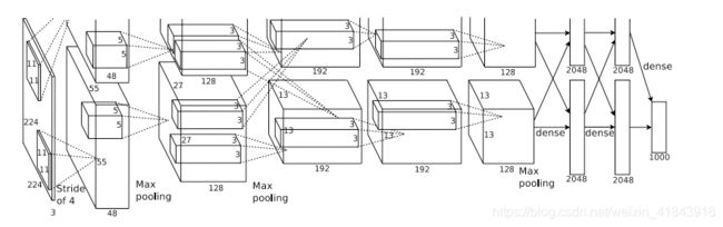
简单说明：

• 1.conv1层，使用较大的11 x 11窗口来捕获物体。同时使用步幅 4 来较大幅度减小输出高和宽。这里使用的输出通道为48，比LeNet的通道数多很多。

• 2.max1层，池化核尺寸为3 x 3，步幅为2，减小卷积的窗口

• 3.conv2层，卷积核尺寸为5 x 5，使用填充为padding = 2来使得输入与输出的高和宽一致，且增大了输出通道数。

• 4.max2层，池化核尺寸为3 x 3，步幅为2，减小卷积的窗口

• 5.conv3层，卷积核尺寸为3 x 3，步幅为1，自动填充

• 6.conv4层，卷积核尺寸为3 x 3，步幅为1，自动填充

• 7.conv5层，卷积核尺寸为3 x 3，步幅为1，自动填充

• 8.max3层，池化核尺寸为3 x 3，步幅为2，减小卷积的窗口

• 9.fc1、fc2层，全连接层的输出个数比LeNet中的大数倍，使用dropout来缓解过拟合

• 10.fc3输出层，根据需要输出类别个数。

• 下面给出基于Keras的一个实现

def AlexNet():
	# 定义模型
    model = Sequential()
    # conv1，卷积核11 * 11，步长4，第一层要指定输入的形状
    model.add(Conv2D(96,(11,11),strides=(4,4),input_shape=(227,227,3),padding='valid',activation='relu',kernel_initializer='uniform'))
    # Max1，池化核3 * 3，步长2
    model.add(MaxPooling2D(pool_size=(3,3),strides=(2,2)))
    # conv2，卷积核5 * 5，自动padding
    model.add(Conv2D(256,(5,5),strides=(1,1),padding='same',activation='relu',kernel_initializer='uniform'))
    # Max2，池化核3 * 3 ，步长2
    model.add(MaxPooling2D(pool_size=(3,3),strides=(2,2)))
    # conv3，卷积核 3 * 3，步长1，连续3个卷积层
    model.add(Conv2D(384,(3,3),strides=(1,1),padding='same',activation='relu',kernel_initializer='uniform'))
    model.add(Conv2D(384,(3,3),strides=(1,1),padding='same',activation='relu',kernel_initializer='uniform'))
    model.add(Conv2D(256,(3,3),strides=(1,1),padding='same',activation='relu',kernel_initializer='uniform'))
    # Max3，池化核3 * 3，步长2
    model.add(MaxPooling2D(pool_size=(3,3),strides=(2,2)))
    # 向量化
    model.add(Flatten())
    # FC1，全连接，后面紧接一个dropout，降低复杂度
    model.add(Dense(4096,activation='relu'))
    model.add(Dropout(0.5))
    # FC2， 全连接
    model.add(Dense(4096,activation='relu'))
    model.add(Dropout(0.5))
    # FC3，输出层，多分类softmax作用
    model.add(Dense(1000,activation='softmax'))
    return model

【概括】

• AlexNet跟LeNet的结构类似，但是使用了更多的卷积层和更大的参数空间来拟合大规模数据集，它是浅层神经网络和深度神经网络的分界线。
• 虽然看上去AlexNet的实现比LeNet的实现也就多了几行代码，但这个观念上的转变和真正优秀实验结果的产生令学术界付出了很多年的努力。

8.使用重复元素的网络（VGG-Nets）

AlexNet在LeNet的基础之上增加了3个卷积层。但AlexNet作者对他们的卷积窗口、输出通道数和构造顺序做了大量的调整。虽然AlexNet指明了深度卷积神经网络可以取得出色的结果，但并没有提供简单的规则以指导后来的研究者如何设计新的网络。
下面提到的VGG网络结构，提出了可以通过重复使用简单的基础块来构建深度模型的思路。

【VGG块】

• 前面说到VGG是通过重复使用简单的基础块构成，那么这个基础块就是VGG块。
• VGG块的组成规律是：连续使用数个相同的填充为1、窗口形状为3 x 3的卷积层后接上一个步幅为2、窗口形状为2 x 2的最大池化层。
• 卷积层保持输入的高和宽不变，而池化层则对其进行减半。

【VGG网络模型】

• VGG-Nets网络的来源是，英国牛津大学的一个实验室Visual Geometry Group。
• 在2014年的ImageNet图像大赛的定位任务和分类任务中分别斩获了冠军和亚军。
• VGG可以看做是AlexNet的加深版本，都是conv layer + FC layer，在当时看来是一个非常深的网络结构了，因为层数多达十几层，当然现在看来已经算不上什么了。
• 下面看一下网络的构成。

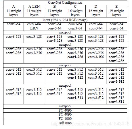
对上述的VGG网络构成简单说明：

• 上面就是整个VGG网络的诞生过程。
• 为了解决参数初始化（权重初始化）问题，VGG采用了“预训练”的方式，这种训练方式在经典的神经网络中经常见到
• 先训练一部分小网络，然后在确定这部分网络稳定之后，在这基础之上再加深网络。在上述的表格中就是这样的一个过程，并且经过大量的实验，发现在D阶段的效果是最好的，而这个阶段conv层 + FC层整好是16层（不包括maxpooling层），因此这个结构就被称作：VGG-16。
• 下面看一下这个VGG-16

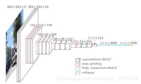
对VGG-16网络结构简单说明：

• 上述的网络结构不再逐层分析，大致是前面的卷积部分和后面的全连接部分，而全连接部分也是平移了AlexNet的3层全连接。

• VGG的特点：

  • 小卷积核。设计者将卷积核全部替换为3 x 3，少数部分用到了1 x 1。
  • 小池化核。相比于AlexNet的3 x 3的卷积核，全部使用的2 x 2。
  • 层数更深特征图更宽。基于前两点外，由于卷积核专注于扩大通道数、池化专注于缩小宽和高，使得模型架构上更深更宽的同时，计算量的增加放缓；
  • 全连接转卷积。网络测试阶段将训练阶段的三个全连接替换为三个卷积，测试重用训练时的参数，使得测试得到的全卷积网络因为没有全连接的限制，因而可以接收任意宽或高为的输入。

• 小卷积核的有点：

  • 多个小卷积核比一个大卷积核有更多的非线性。使得判决函数更加具有判决性。
  • 多个小卷积核与一个大的卷积核的计算参数相差无几，但是计算量却是大大增加。
  • 大卷积核的计算量比较大。
  • 1 x 1的卷积核，可以在不影响输入和输出维度的前提下，对输入进行线性变换，然后通过ReLU进行非线性变换，增加网络的非线性表达能力。

• 下面给出基于Keras的一个实现

def VGG_16():   
	# 定义模型
    model = Sequential()
    
    # vgg_block1，2个卷积层，后面接一个池化
    model.add(Conv2D(64,(3,3),strides=(1,1),input_shape=(224,224,3),padding='same',activation='relu',kernel_initializer='uniform'))
    model.add(Conv2D(64,(3,3),strides=(1,1),padding='same',activation='relu',kernel_initializer='uniform'))
    model.add(MaxPooling2D(pool_size=(2,2)))
    
    # vgg_block2，2个卷积层，后面接一个池化
    model.add(Conv2D(128,(3,2),strides=(1,1),padding='same',activation='relu',kernel_initializer='uniform'))
    model.add(Conv2D(128,(3,3),strides=(1,1),padding='same',activation='relu',kernel_initializer='uniform'))
    model.add(MaxPooling2D(pool_size=(2,2)))
    
    # vgg_block3，3个卷积层，后面接一个池化
    model.add(Conv2D(256,(3,3),strides=(1,1),padding='same',activation='relu',kernel_initializer='uniform'))
    model.add(Conv2D(256,(3,3),strides=(1,1),padding='same',activation='relu',kernel_initializer='uniform'))
    model.add(Conv2D(256,(3,3),strides=(1,1),padding='same',activation='relu',kernel_initializer='uniform'))
    model.add(MaxPooling2D(pool_size=(2,2)))
    
    # vgg_block4，3个卷积层，后面接一个池化
    model.add(Conv2D(512,(3,3),strides=(1,1),padding='same',activation='relu',kernel_initializer='uniform'))
    model.add(Conv2D(512,(3,3),strides=(1,1),padding='same',activation='relu',kernel_initializer='uniform'))
    model.add(Conv2D(512,(3,3),strides=(1,1),padding='same',activation='relu',kernel_initializer='uniform'))
    model.add(MaxPooling2D(pool_size=(2,2)))
    
    # vgg_block5，3个卷积层，后面接一个池化
    model.add(Conv2D(512,(3,3),strides=(1,1),padding='same',activation='relu',kernel_initializer='uniform'))
    model.add(Conv2D(512,(3,3),strides=(1,1),padding='same',activation='relu',kernel_initializer='uniform'))
    model.add(Conv2D(512,(3,3),strides=(1,1),padding='same',activation='relu',kernel_initializer='uniform'))
    model.add(MaxPooling2D(pool_size=(2,2)))
    
    model.add(Flatten())
	
	# 2个FC层，隐藏层
    model.add(Dense(4096,activation='relu'))
    model.add(Dropout(0.5))
    model.add(Dense(4096,activation='relu'))
    model.add(Dropout(0.5))
	
	# 1个FC层，输出层
    model.add(Dense(1000,activation='softmax'))
    
    return model

【概括】

• VGG-16通过多个可以重复使用卷积块来构造网络。根据每块里卷积层个数和输出通道数的不同可以定义出不同的VGG模型。

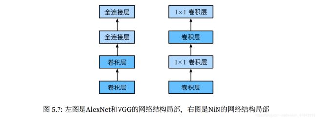
9.网络中的网络（NiN）

前面介绍了LeNet、AlexNet、VGG网络结构，三者在设计上的共同之处是：先以由卷积层构成的模块充分抽取空间特征，再以由全连接层构成的模块来输出分类结果（简单说就是：卷积层+全连接层）。其中，AlexNet和VGG对LeNet的改进主要在于如何对这两个模块加宽（增加通道数）和加深（增加层）。下面介绍的NiN（Network in Network）网络，它提出了另外的一个思路，即串联多个由卷积层和“全连接”层构成的小网络来构建一个深层网络。
【两个重要概念】

• 1 x 1卷积的作用：
  • 1.实现跨通道的交互和信息整合。
  • 2.进行卷积核通道数的降维和升维。
  • 说明：在NiN网络中这个应用很多，就是用多层卷积网络（MLP）代替传统卷积层。
• 全局平均池化
  • 1.使用平均池化代替全连接
  • 2.很大程度上减少参数空间，便于加深网络和训练，有效降低过拟合。

【NiN块】

• 我们知道，在卷积层的输入和输出通常是4维的数组（样本，通道，高，宽）；而全连接层的输入和输出则通常是二维数组（样本，特征）。如果想在全连接层后在接上卷积层，则需要将全联机的输出变换成4维。
• 在前面介绍“多输入通道和多输出通道”时，提到了1 x 1卷积层。他可以看成全连接层，其中空间维度（高和宽）上的每个元素相当于样本，通道相当于特征。因此，NiN使用1 x 1 卷积层来替代全连接层，从而使空间信息能够自然传递到后面的层中去。看下图说明：

• NiN块是NiN中的基础块。它由一个卷积层加两个充当全连接层的1 x 1卷积层串联而成。其中第一个卷积层的超参数可以自行配置，而第二个和第三个卷积层的超参数一般是固定的。
• 下面使用MXNet库进行代码实现说明：

from mxnet import gluon,init,nd
from mxnet.gluon import nn
def nin_block(num_channels,kernel_size,strides,padding):
    """
    构建一个NiN块，这个块也叫做MLPconv（多层感知卷积层），其实就是：传统卷积层+1 x 1卷积层。
    用这个NiN块代替传统卷积可以增强网络提取抽象特征和泛化能力。
    
    Parameters:
    ----------------
    num_channels:通道数，也就是卷积后的厚度
    kernel_size:卷积核的形状
    strides:步幅
    padding:填充
    
    return:
    ----------------
    blk:定义好的一个mlpconv结构
    """

    blk = nn.Sequential()
    blk.add(nn.Conv2D(num_channels,kernel_size,strides,padding,activation = 'relu'),
            nn.Conv2D(num_channels,kernel_size = 1,activation = 'relu'),
            nn.Conv2D(num_channels,kernel_size = 1,activation = 'relu'))
    return blk

【NiN模型】
NiN是AlexNet问世不久后提出的。他们的卷积层设定有类似之处。NiN使用卷积窗口形状分别为11 x 11、5 x 5和3 x 3 的卷积层，相应的输出通道数也与AlexNet中的一致。每个NiN块后接一个步幅为2、窗口形状为3 x 3的最大池化层。
除了使用NiN块以外NiN还有一个设计与AlexNet显著不同：NiN去掉了AlexNet最后的3个全连接层，取而代之的，NiN使用了输出通道数 = 标签类别数的NiN块，然后使用全局平均池化层对每个通道中所有元素求平均并直接用于分类。这里的全军平均池化层即窗口形状等于输入空间维度形状的平均池化层。NiN的这个设计的好处是可以显著减小模型参数尺寸，从而缓解过拟合。然而该设计有时会造成获得有效模型的训练时间的增加。

• 下面使用MXNet库进行代码实现说明：

net = nn.Sequential()
# 前面的卷积层部分，用mlpconv代替了传统的方式；后面的全连接部分用NiN块结合全局平均处理
net.add(nin_block(96,kernel_size = 11,strides = 4,padding = 0),
       nn.MaxPool2D(pool_size = 3,strides = 2),
       nin_block(256,kernel_size=5,strides = 1,padding =2),
       nn.MaxPool2D(pool_size = 3,strides = 2),
       nin_block(384,kernel_size = 3,strides = 1,padding = 1),
       nn.MaxPool2D(pool_size = 3,strides =2),
       nn.Dropout(0.5),

	   # 后面部分就是AlexNet的'全连接部分'
       # 类别标签，类别数为10，因为使用的手写体
       nin_block(10,kernel_size = 3,strides = 1,padding = 1),
       # 全局平均池化层将窗口形状自动设置为输入的高和宽
       nn.GlobalAvgPool2D(),
       # 将四维的输入转化成二维的输出，其形状为（批量大小，10）
       nn.Flatten())

• 下面构建一个数据样本来查看一下每层的输出形状。

X = nd.random.uniform(shape=(1,1,244,244))
net.initialize()
for layer in net:
    X = layer(X)
    print(layer.name,'output shape :\t',X.shape)

[out]:sequential6 output shape :	 (1, 96, 59, 59)
	  pool4 output shape :	 (1, 96, 29, 29)
	  sequential7 output shape :	 (1, 256, 29, 29)
	  pool5 output shape :	 (1, 256, 14, 14)
	  sequential8 output shape :	 (1, 384, 14, 14)
	  pool6 output shape :	 (1, 384, 6, 6)
	  dropout1 output shape :	 (1, 384, 6, 6)
	  sequential9 output shape :	 (1, 10, 6, 6)
	  pool7 output shape :	 (1, 10, 1, 1)
	  flatten1 output shape :	 (1, 10)

• 使用Fashion - MNIST数据集来训练模型。NiN的训练与AlexNet和VGG的类似，但这里使用的学习率更大。

from mxnet.gluon import data as gdata
import mxnet as mx
from mxnet.gluon import loss as gloss,nn
import os
import sys
import time
# 需要定义几个函数
def load_data_fashion_mnist(batch_size, resize=None, root=os.path.join('~', '.mxnet', 'datasets', 'fashion-mnist')):
	"""
	用于加载‘fashion-mnist’数据集，并返回一定批次的训练集和测试集
	"""
    root = os.path.expanduser(root)  # 展开用户路径'~'
    transformer = []
    if resize:
        transformer += [gdata.vision.transforms.Resize(resize)]
    transformer += [gdata.vision.transforms.ToTensor()]
    transformer = gdata.vision.transforms.Compose(transformer)
    mnist_train = gdata.vision.FashionMNIST(root=root, train=True)
    mnist_test = gdata.vision.FashionMNIST(root=root, train=False)
    num_workers = 0 if sys.platform.startswith('win32') else 4
    train_iter = gdata.DataLoader(
        mnist_train.transform_first(transformer), batch_size, shuffle=True,
        num_workers=num_workers)
    test_iter = gdata.DataLoader(
        mnist_test.transform_first(transformer), batch_size, shuffle=False,
        num_workers=num_workers)
    return train_iter, test_iter


def try_gpu():  
	"""
	如果有GPU就优先使用，否则使用CPU
	"""
    try:
        ctx = mx.gpu()
        _ = nd.zeros((1,), ctx=ctx)
        print('use gpu')
    except mx.base.MXNetError:
        ctx = mx.cpu()
        print('use cpu')
    return ctx

def evaluate_accuracy(data_iter, net, ctx):
	"""
	用于评估模型
	"""
    acc_sum, n = nd.array([0], ctx=ctx), 0
    for X, y in data_iter:
        # 如果ctx代表GPU及相应的显存，将数据复制到显存上
        X, y = X.as_in_context(ctx), y.as_in_context(ctx).astype('float32')
        acc_sum += (net(X).argmax(axis=1) == y).sum()
        n += y.size
    return acc_sum.asscalar() / n


def train_ch5(net, train_iter, test_iter, batch_size, trainer, ctx,num_epochs):
	"""
	定义训练器
	"""
    print('training on', ctx)
    loss = gloss.SoftmaxCrossEntropyLoss()
    for epoch in range(num_epochs):
        train_l_sum, train_acc_sum, n, start = 0.0, 0.0, 0, time.time()
        for X, y in train_iter:
            X, y = X.as_in_context(ctx), y.as_in_context(ctx)
            with autograd.record():
                y_hat = net(X)
                l = loss(y_hat, y).sum()
            l.backward()
            trainer.step(batch_size)
            y = y.astype('float32')
            train_l_sum += l.asscalar()
            train_acc_sum += (y_hat.argmax(axis=1) == y).sum().asscalar()
            n += y.size
        test_acc = evaluate_accuracy(test_iter, net, ctx)
        print('epoch %d, loss %.4f, train acc %.3f, test acc %.3f, '
              'time %.1f sec'
              % (epoch + 1, train_l_sum / n, train_acc_sum / n, test_acc,
                 time.time() - start))

##############################
# 开始训练
# 定义参数
lr,num_epochs,batch_size,ctx  = 0.1,5,128,try_gpu()
# 初始化参数，初始化方式：Xavier
net.initialize(force_reinit= True,init=init.Xavier())
# 初始化训练器
trainer = gluon.Trainer(net.collect_params(),'sgd',{'learning_rate':lr})
# 加载数据集
train_iter,test_iter = load_data_fashion_mnist(batch_size,resize = 224)
# 训练模型
train_ch5(net,train_iter,test_iter,batch_size,trainer,ctx,num_epochs)


[out]:training on gpu(0)
	  epoch 1, loss 2.2493, train acc 0.190, test acc 0.373, time 24.4 sec
	  epoch 2, loss 1.7309, train acc 0.353, test acc 0.539, time 23.3 sec
	  epoch 3, loss 0.8903, train acc 0.659, test acc 0.761, time 23.4 sec
	  epoch 4, loss 0.6465, train acc 0.760, test acc 0.805, time 23.3 sec
	  epoch 5, loss 0.5096, train acc 0.812, test acc 0.831, time 23.3 sec

【三种网络结构】

• 传统的卷积层（convolution）

• 单通道mplconv层

• 跨通道mplconv层（cccp层）

• 由上图可以发现，mlpconv = convolution + mlp
• 在caffe中的实现，mplconv = convolution + 1×1convolution+1×1convolution（2层的mlp）

• 由于概念比较难以理解，借用一张图解释CNN、Maxout、MLP的区别。

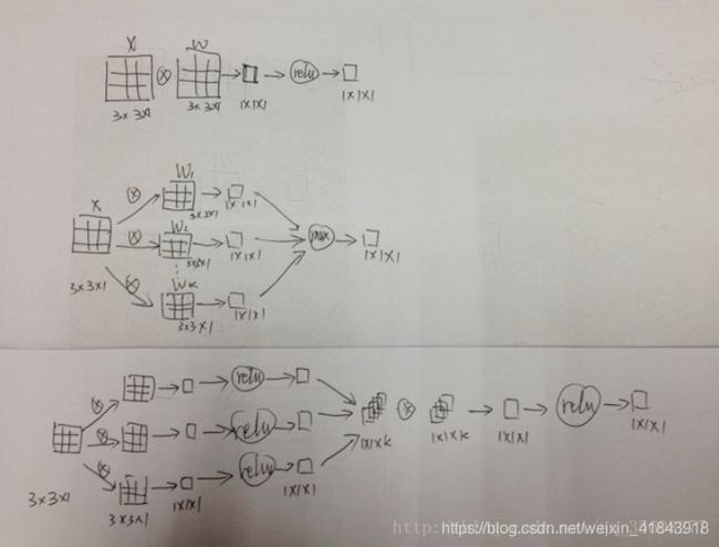
• Maxout 和MLP都是对传统CNN的改进：
  • Maxout想表明它可以拟合任意的凸函数，也就能够拟合任意的激活函数（默认激活函数都是凸函数）
  • NIN想表明它不仅能够拟合任何凸函数，而且能够拟合任何函数，因为它本质上可以说是一个小型的全连接神经网络。

【概括】

• NiN重复使用由卷积层和代替全连接层的1 x 1 卷积层构成的NiN块来构建深层网络。
• NiN去除了容易造成过拟合的全输出层，而是将其替换成输出通道数等于标签类别数的NiN块和全局平均池化层。
• NiN的以上设计思想影响了后面一系列卷积神经网络的设计。

10.含并行连接的网络（GoogLeNet）

在2014年的ImageNet图像识别挑战赛中，一个叫做GoogLeNet的网络结构大放异彩。它虽然在名字上想LeNet致敬，但在网络结构上已经很难看到LeNet的影子了。GoogLeNet吸收了NiN中网络串联网络的思想，并在此基础上做了很大改进。在随后的几年里，研究人员对GoogLeNet进行了数次改进。下面介绍这个模型系列的第一个版本。

【Inception块】

• GoogLeNet中的基础卷积块叫作Inception块，得名于同名电影《盗梦空间》（Inception）。与上一节介绍的NiN块相比，这个基础在结构上更加复杂，如下图。

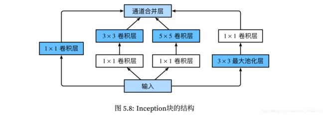
• 由图可以看到，Inception块里有4条并行的线路。前3条线路使用的窗口大小分别是1 x 1、3 x 3 和5 x 5 的卷积层来抽取不同空间尺寸下的信息，其中中间2个线路会对输入先做1 x 1卷积来减少输入通道数，以降低模型复杂度。第四条线路则使用3 x 3最大池化层，后接1 x 1卷积层来改变通道数。4条线路都使用了合适的填充来使得输入与输出的高和宽一致。最后我们将每条线路的输出在通道维上连结，并输入接下来的层中去。
• 代码实现

from mxnet import gluon, init, nd
from mxnet.gluon import nn
class Inception(nn.Block):
	# c1 - c4为每条线路⾥的层的输出通道数
	def __init__(self, c1, c2, c3, c4, **kwargs):
		super(Inception, self).__init__(**kwargs)
		# 线路1，单1 x 1卷积层
		self.p1_1 = nn.Conv2D(c1, kernel_size=1, activation='relu')
		# 线路2， 1 x 1卷积层后接3 x 3卷积层
		self.p2_1 = nn.Conv2D(c2[0], kernel_size=1, activation='relu')
		self.p2_2 = nn.Conv2D(c2[1], kernel_size=3, padding=1,activation='relu')
		# 线路3， 1 x 1卷积层后接5 x 5卷积层
		self.p3_1 = nn.Conv2D(c3[0], kernel_size=1, activation='relu')
		self.p3_2 = nn.Conv2D(c3[1], kernel_size=5, padding=2,activation='relu')
		# 线路4， 3 x 3最⼤池化层后接1 x 1卷积层
		self.p4_1 = nn.MaxPool2D(pool_size=3, strides=1, padding=1)
		self.p4_2 = nn.Conv2D(c4, kernel_size=1, activation='relu')
	def forward(self, x):
		p1 = self.p1_1(x)
		p2 = self.p2_2(self.p2_1(x))
		p3 = self.p3_2(self.p3_1(x))
		p4 = self.p4_2(self.p4_1(x))
		return nd.concat(p1, p2, p3, p4, dim=1) # 在通道维上连结输出

【GoogLeNet模型】

• GoogLeNet跟VGG一样，在主题卷积部分中使用了5个模块（block）,每个模块之间使用步幅维的3 x 3最大池化层来减小输出高宽。第一模块使用了64通道的7 x 7卷积层。

b1 = nn.Sequential()
b1.add(nn.Conv2D(64,kernel_size = 7,strides = 2,padding = 3,activation = 'relu'),
	   nn.MaxPool2D(poo_size = 3,strides = 2,padding = 1))

• 第二模块使用2个卷积层：首先是64通道的1 x 1卷积层，然后是将通道增大3倍的3 x 3卷积层。他对应Inception块中的第二条线路。

b2 = nn.Sequential()
b2.add(nn.Conv2D(64,kernel_size = 1,activation = 'relu'),
 			nn.Conv2D(192,kernel_size = 3,padding = 1,activation = 'relu'),
 			nn.MaxPool2D(pool_size = 3,strides = 2,padding = 1))

• 第三模块串联2个完整的Inception块。第一个Inception块的输出64 + 128 + 32 + 32 = 256，其中4条线路的输出通道数比例为64:128:32:32 = 2:4:1:1。其中第二、第三条线路分别将输入通道数减小至96/192 = 1/2和16/192 = 1/12后，在街上第二层卷积层。第二个Inception块输出通道数增值128 + 192 + 96 + 64 = 480，每条线路的输出通道数之比为128:192:96:64 = 4:6:3:2。其中第二、第三条线路先分别将输入通道数减小至128/256 = 1/2和32/256 = 1/8.

b3 = nn.Sequential()
b3.add(Inception(64,(96,128),(16,32),32),
	   Inception(129,(128,192),(32,96),64,)
	   nn.MaxPool2D(pool_size = 3,stides = 2,padding = 1))

• 第四个模块更加复杂。它串联了5个Inception块，其输出通道数分别是192 + 208 + 48 + 64 = 512、160+224+64+64 = 512、128+256+64+64 = 512、112+288+64+64 = 528和256+320+128+128 =832。这些线路的通道数分配和第三模块中的类似，⾸先含3 × 3卷积层的第⼆条线路输出最多通道，其次是仅含1× 1卷积层的第⼀条线路，之后是含5× 5卷积层的第三条线路和含3× 3最⼤池化层的第四条线路。其中第⼆、第三条线路都会先按⽐例减小通道数。这些⽐例在各个Inception块中都略有不同

b4 = nn.Sequential()
b4.add(Inception(192, (96, 208), (16, 48), 64),
	   Inception(160, (112, 224), (24, 64), 64),
	   Inception(128, (128, 256), (24, 64), 64),
	   Inception(112, (144, 288), (32, 64), 64),
	   Inception(256, (160, 320), (32, 128), 128),
	   nn.MaxPool2D(pool_size=3, strides=2, padding=1))

• 第五模块有输出通道数为256 + 320 + 128 + 128 = 832和384 + 384 + 128 + 128 = 1024的两个Inception块。其中每条线路的通道数的分配思路和第三、第四模块中的⼀致，只是在具体数值上有所不同。需要注意的是，第五模块的后⾯紧跟输出层，该模块同NiN⼀样使⽤全局平均池化层来将每个通道的⾼和宽变成1。最后我们将输出变成⼆维数组后接上⼀个输出个数为标签类别数的全连接层。

b5 = nn.Sequential()
b5.add(Inception(256, (160, 320), (32, 128), 128), 
	   Inception(384, (192, 384), (48, 128), 128),
	   nn.GlobalAvgPool2D())
	   net = nn.Sequential()
	   net.add(b1, b2, b3, b4, b5, nn.Dense(10))

• Keras实现

def Conv2d_BN(x, nb_filter,kernel_size, padding='same',strides=(1,1),name=None):
    if name is not None:
        bn_name = name + '_bn'
        conv_name = name + '_conv'
    else:
        bn_name = None
        conv_name = None

    x = Conv2D(nb_filter,kernel_size,padding=padding,strides=strides,activation='relu',name=conv_name)(x)
    x = BatchNormalization(axis=3,name=bn_name)(x)
    return x

def Inception(x,nb_filter):
    branch1x1 = Conv2d_BN(x,nb_filter,(1,1), padding='same',strides=(1,1),name=None)

    branch3x3 = Conv2d_BN(x,nb_filter,(1,1), padding='same',strides=(1,1),name=None)
    branch3x3 = Conv2d_BN(branch3x3,nb_filter,(3,3), padding='same',strides=(1,1),name=None)

    branch5x5 = Conv2d_BN(x,nb_filter,(1,1), padding='same',strides=(1,1),name=None)
    branch5x5 = Conv2d_BN(branch5x5,nb_filter,(1,1), padding='same',strides=(1,1),name=None)

    branchpool = MaxPooling2D(pool_size=(3,3),strides=(1,1),padding='same')(x)
    branchpool = Conv2d_BN(branchpool,nb_filter,(1,1),padding='same',strides=(1,1),name=None)

    x = concatenate([branch1x1,branch3x3,branch5x5,branchpool],axis=3)

    return x

def GoogLeNet():
    inpt = Input(shape=(224,224,3))
    #padding = 'same'，填充为(步长-1）/2,还可以用ZeroPadding2D((3,3))
    x = Conv2d_BN(inpt,64,(7,7),strides=(2,2),padding='same')
    x = MaxPooling2D(pool_size=(3,3),strides=(2,2),padding='same')(x)
    x = Conv2d_BN(x,192,(3,3),strides=(1,1),padding='same')
    x = MaxPooling2D(pool_size=(3,3),strides=(2,2),padding='same')(x)
    x = Inception(x,64)#256
    x = Inception(x,120)#480
    x = MaxPooling2D(pool_size=(3,3),strides=(2,2),padding='same')(x)
    x = Inception(x,128)#512
    x = Inception(x,128)
    x = Inception(x,128)
    x = Inception(x,132)#528
    x = Inception(x,208)#832
    x = MaxPooling2D(pool_size=(3,3),strides=(2,2),padding='same')(x)
    x = Inception(x,208)
    x = Inception(x,256)#1024
    x = AveragePooling2D(pool_size=(7,7),strides=(7,7),padding='same')(x)
    x = Dropout(0.4)(x)
    x = Dense(1000,activation='relu')(x)
    x = Dense(1000,activation='softmax')(x)
    model = Model(inpt,x,name='inception')
    return model

【概括】

• Inception块相当于一个有4条线路的子网络。它通过不同窗口形状的卷积层和最大池化层来并行抽取信息，并使用1 x 1 卷积层减少通道数，从而降低模型复杂度。
• GoogLeNet将多个设计精细的Inception块和其他层串联起来，其中Inception块的通道数分配之比ImageNet数据集上通过大量的实验得来的。
• GoogLeNet和它的后继这们一度是ImageNet上最高效的模型之一：在类似的测试精度下，它们的计算复杂度往往更低。

11.残差网络（ResNet）

先让我们思考一个问题，对于神经网络模型添加新的层，充分训练后的模型是否只可能更有更有效地降低训练误差？理论上，原模型解的空间只是新模型解的空间的子空间。也就是说，如果我们能将新添加的层训练成恒等映射$f(x)=x$，新模型和原模型将同样有效。由于新模型可能得出更优 的解来拟合训练数据，因此添加层似乎更容易降低训练误差。然而在实践中，添加过多的层后训练误差往往不降反升。即使利用批量归一化带来的数值稳定性使训练深层模型更加容易。该问题仍然存在。
针对这一问题，何凯明等人提出了残差网络（ResNet）,它在2015年的ImageNet图像识别赛夺冠，并深刻影响了后来的深度神经网络的设计。

【残差块】
让我们聚焦于神经网络局部。如下图，设输入为$x$。假设我们希望学出的理想映射为$f(x)$。从而作为下图5.9上方激活函数的输入。左图虚线框中的部分需要直接拟合出该映射$f(x)$，而右图虚线框中的部分则需要拟合出有关恒等映射的残差映射$f(x)-x$。残差映射在实际中往往更容易优化。
以本节开头提到的恒等映射作为我们希望学出的理想映射$f(x)$。我们只需要将图5.9中右图虚线框内上方的加权运算（如仿射）的权重和偏差学成0，那么$f(x)$即为恒等映射。图5.9右图也是ResNet的基础块，即残差快（residual block）。在残差快中，输入可通过跨层的数据线路更快地向前传播。

ResNet沿用了VGG全3 x 3卷积层的设计。残差块里首先由2个相同输出通道数的3 x 3卷积层。每个卷积层后接一个批量归一化层和ReLU激活函数。然后我们将输入跳过这个两个卷积层后直接加在最后的ReLU激活函数前。这样的设计要求两个卷积层的输出与输入形状一样，从而可以相加。如果想要改变通道数，就需要引入一个额外的1 x 1卷积层来将输入变成需要的形状后再做相加运算。
残差块的实现如下，它可以设定输出通道、是否使用额外的1 x 1卷积层来修改通道数以及卷积层的步幅。

from mxnet.gluon import nn
from mxnet import gluon,init,nd
class Residual(nn.Block):
    def __init__(self,num_channels,use_1x1conv = False,strides = 1,**kwargs):
        super(Residual,self).__init__(**kwargs)
        self.conv1 = nn.Conv2D(num_channels,kernel_size=3,padding=1,strides=strides)
        self.conv2 = nn.Conv2D(num_channels,kernel_size=3,padding=1)
        if use_1x1conv:
            self.conv3 = nn.Conv2D(num_channels,kernel_size=1,strides=strides)
        else:
            self.conv3 = None
        self.bn1 = nn.BatchNorm()
        self.bn2 = nn.BatchNorm()
    def forward(self,X):
        Y = nd.relu(self.bn1(self.conv1(X)))
        Y = self.bn2(self.conv2(Y))
        if self.conv3:
            X = self.conv3
        return nd.relu(Y + X)

【ResNet模型】

• ResNet的前两层跟之前介绍的GoogLeNet中的⼀样：在输出通道数为64、步幅为2的7 × 7卷积层后接步幅为2的3 × 3的最⼤池化层。不同之处在于ResNet每个卷积层后增加的批量归⼀层。

net = nn.Sequential()
net.add(nn.Conv2D(64, kernel_size=7, strides=2, padding=3),
        nn.BatchNorm(), 
        nn.Activation('relu'),
        nn.MaxPool2D(pool_size=3, strides=2, padding=1))

• GoogLeNet在后⾯接了4个由Inception块组成的模块。 ResNet则使⽤4个由残差块组成的模块，每个模块使⽤若⼲个同样输出通道数的残差块。第⼀个模块的通道数同输⼊通道数⼀致。由于之前已经使⽤了步幅为2的最⼤池化层，所以⽆须减小⾼和宽。之后的每个模块在第⼀个残差块⾥将上⼀个模块的通道数翻倍，并将⾼和宽减半。
• 下面我们来实现这个模块。注意，这里对第一个模块做了特别处理。

def resnet_block(num_channels, num_residuals, first_block=False):
    blk = nn.Sequential()
    for i in range(num_residuals):
        if i == 0 and not first_block:
            blk.add(Residual(num_channels, use_1x1conv=True, strides=2))
        else:
        blk.add(Residual(num_channels))
    return blk

• 接着我们为ResNet加⼊所有残差块。这⾥每个模块使⽤两个残差块。

net.add(resnet_block(64, 2, first_block=True),
        resnet_block(128, 2),
        resnet_block(256, 2),
        resnet_block(512, 2))

• 最后，与GoogLeNet⼀样，加⼊全局平均池化层后接上全连接层输出。

net.add(nn.GlobalAvgPool2D(), nn.Dense(10))

• 这⾥每个模块⾥有4个卷积层（不计算1 × 1卷积层），加上最开始的卷积层和最后的全连接层，共计18层。这个模型通常也被称为ResNet-18。通过配置不同的通道数和模块⾥的残差块数可以得到不同的ResNet模型，例如更深的含152层的ResNet-152。虽然ResNet的主体架构跟GoogLeNet的类似，但ResNet结构更简单，修改也更⽅便。这些因素都导致了ResNet迅速被⼴泛使⽤。

【概括】

• 残差块通过跨层的数据通道从而能够训练处有效的深度神经网络。
• ResNet深刻影响了后来的深度神经⽹络的设计。

12.稠密连接网络（DenseNet）

ResNet中的跨层连接设计引申出了数个后续⼯作。本节我们介绍其中的⼀个：稠密连接⽹络
（DenseNet）。它与ResNet的主要区别如图5.10所⽰。

• 图5.10中将部分前后相邻的运算抽象为模块A和模块B。与ResNet的主要区别在于， DenseNet⾥模块B的输出不是像ResNet那样和模块A的输出相加，而是在通道维上连结。这样模块A的输出可以直接传⼊模块B后⾯的层。在这个设计⾥，模块A直接跟模块B后⾯的所有层连接在了⼀起。这也是它被称为“稠密连接”的原因。
• DenseNet的主要构建模块是稠密块（ dense block）和过渡层（ transition layer）。前者定义了输⼊和输出是如何连结的，后者则⽤来控制通道数，使之不过⼤。

【稠密块】

• DenseNet使⽤了ResNet改良版的“批量归⼀化、激活和卷积”结构（参⻅上⼀节的练习），我们⾸先在conv_block函数⾥实现这个结构。

from mxnet import gluon, init, nd
from mxnet.gluon import nn
def conv_block(num_channels):
    blk = nn.Sequential()
    blk.add(nn.BatchNorm(), 
            nn.Activation('relu'),
            nn.Conv2D(num_channels, kernel_size=3, padding=1))
    return blk

• 稠密块由多个conv_block组成，每块使⽤相同的输出通道数。但在前向计算时，我们将每块的
  输⼊和输出在通道维上连结。

class DenseBlock(nn.Block):
    def __init__(self, num_convs, num_channels, **kwargs):
        super(DenseBlock, self).__init__(**kwargs)
        self.net = nn.Sequential()
        for _ in range(num_convs):
            self.net.add(conv_block(num_channels))
    def forward(self, X):
        for blk in self.net:
            Y = blk(X)
            X = nd.concat(X, Y, dim=1) # 在通道维上将输⼊和输出连结
        return X

【过渡层】
由于每个稠密块都会带来通道数的增加，使⽤过多则会带来过于复杂的模型。过渡层⽤来控制模型复杂度。它通过1 × 1卷积层来减小通道数，并使⽤步幅为2的平均池化层减半⾼和宽，从而进⼀步降低模型复杂度。

def transition_block(num_channels):
    blk = nn.Sequential()
    blk.add(nn.BatchNorm(),
            nn.Activation('relu'),
            nn.Conv2D(num_channels, kernel_size=1),
            nn.AvgPool2D(pool_size=2, strides=2))
    return blk

【DenseNet】

• 我们来构造DenseNet模型。 DenseNet⾸先使⽤同ResNet⼀样的单卷积层和最⼤池化层。

net = nn.Sequential()
net.add(nn.Conv2D(64, kernel_size=7, strides=2, padding=3),
        nn.BatchNorm(), 
        nn.Activation('relu'),
        nn.MaxPool2D(pool_size=3, strides=2, padding=1))

• 类似于ResNet接下来使⽤的4个残差块， DenseNet使⽤的是4个稠密块。同ResNet⼀样，我们可以设置每个稠密块使⽤多少个卷积层。这⾥我们设成4，从而与上⼀节的ResNet-18保持⼀致。稠密块⾥的卷积层通道数（即增⻓率）设为32，所以每个稠密块将增加128个通道。
• ResNet⾥通过步幅为2的残差块在每个模块之间减小⾼和宽。这⾥我们则使⽤过渡层来减半⾼和宽，并减半通道数。

num_channels, growth_rate = 64, 32 # num_channels为当前的通道数
num_convs_in_dense_blocks = [4, 4, 4, 4]
for i, num_convs in enumerate(num_convs_in_dense_blocks):
    net.add(DenseBlock(num_convs, growth_rate))
    # 上⼀个稠密块的输出通道数
    num_channels += num_convs * growth_rate
    # 在稠密块之间加⼊通道数减半的过渡层
    if i != len(num_convs_in_dense_blocks) - 1:
        num_channels //= 2
        net.add(transition_block(num_channels))

• 同ResNet⼀样，最后接上全局池化层和全连接层来输出。

net.add(nn.BatchNorm(), 
        nn.Activation('relu'), 
        nn.GlobalAvgPool2D(),
        nn.Dense(10))

【概括】

• 在跨层连接上，不同于ResNet中将输入与输出相加，DenseNet在通道维上连结输入与输出。
• DenseNet的主要构件模块是稠密块和过渡层。