DataWhale——机器学习常用算法总结
机器学习笔记
- 一级目录
- 机器学习
-
- 定义
- 分类
-
- 学派分类
- 按照学习方式分类
- 业务领域分类
- 学习步骤
- 学习技巧
- 学习轮次
- 任务
- 按照模型来分
- 机器学习开发流程
-
- 数据集
- 常见数据集
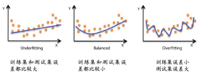
- 误差分析
- 泛化误差分析
-
- 欠拟合:高偏差低方差
- 过拟合:低偏差高方差
- 交叉验证
- 线性回归
- 逻辑回归
- 支持向量机
-
- 遇事不决就加核
- 决策树
-
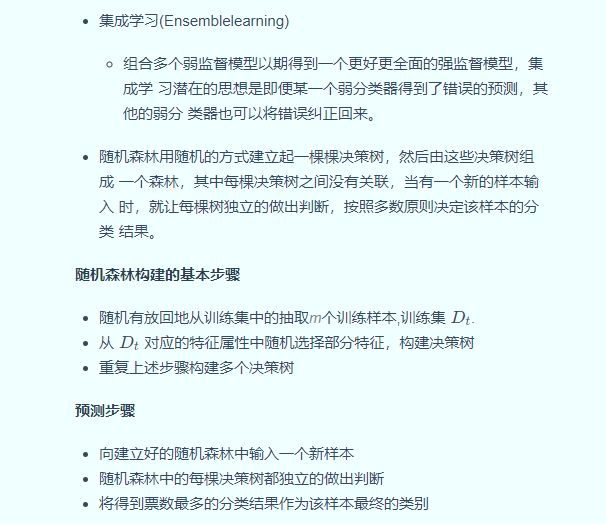
- 随机森林
- 无监督学习
-
- 聚类
- kmeans
- 均值漂移(不需要指定聚类数)
- 层次聚类
- 密度聚类
- 混合高斯聚类
- AP(近邻传播算法affinity propagation )聚类
- 降维
-
- PCA主成分分析(无监督)
- LDA 线性判别分析,有监督降维,也可做分类
一级目录
机器学习
定义
- 让计算机具有像人 一样的学习和思考能力
- 让计算机学会人类的某一项技能
分类
学派分类
- 符号主义
用符号(符号代表的知识)进行逻辑推导(人类认知和思维的基本单元是符号,而认知过程就是在符号表示上的一种运算) - 连接主义 (类似于神经元)
模拟、仿真人类大脑的方式进行推导运算(神经网络、神经元) - 行为主义(进化类)
模拟人类的进化过程
按照学习方式分类
- 有监督
有样本指导,可以判断正误(正误是外在) - 无监督
例如婴儿习得技能、聚类、生成式对抗网络 - 自监督
对样本自行判断然后对照样本正误(正误是内在) - 半监督
业务领域分类
- 信号、无线电
- 图像
- 语音领域
- 自然语义
- 自动化
学习步骤
- 端到端学习
输入–>模型–>输出 - 非端到端学习
输入–>特征提取器–>特征–>分类器–>输出
学习技巧
- 迁移学习
用运用以前学习的知识来学习新的知识 - 元学习
学习概念/本质/原理,之后举一反三 - 级联学习
大块任务分成多个小任务,一个一个学习 - 递增学习
由简单到困难学习 - 对抗学习
竞争的方式学习 - 合作学习
学习轮次
- N-SHOT
多轮次学习
大批量学习
小批量学习 - ONE-SHOT
学习一次 - ZERO-SHOT
触类旁通(由英语翻译汉语+汉语翻译法语 来得知 英语翻译法语的技能)
任务
- 回归/拟合/函数逼近
回归:用模型获得样本的值
拟合:多个样本可以用曲线表达从而推导出公式
函数逼近:样本可以近似用一个函数表达 - 分类
- 聚类
把相同特征的样本聚合在一起,没有分类能力(无监督) - 特征提取/降维/主成分分析
特征提取:提取特征后,可做相似度比较
降维:筛选出重要的特征,容易区分
主成分分析:给特征加权重 - 生成创作
例子:生成一个实际不存在的人的相貌(style GAN2);生成一篇文章 - 评估与规划
规划:规划一个个步骤,然后按照步骤依次实行;例子:ai下围棋
评估:用分值之类判断标准程度;例子:评估相貌90分 - 决策
得到数据样本后,实行具体命令操作
按照模型来分
- 统计
线性回归
最大熵 - 仿生
进化算法
蚁群算法
再提一点,深度学习属于机器学习一个领域,无非自成了体系。
机器学习开发流程
- 模型研发流程
- 数据处理(占用大部分工作内容 约80%)
- 数据采集
人工收集、系统采集、爬虫、虚拟仿真、对抗生成、开源数据 - 数据标注
人工标注、数据标注软件、自动化标注 - 数据清洗
去掉不好的数据 - 数据增强
对数据作增强处理(一个数据增强为多个数据)
增强工具、openCV等编程 - 数据预处理
预处理可以提高模型训练效率
利用好非标注数or数据标注自动化是降低成本的关键
科学采样,体现整体样本的分布规律
数据质量重于数据数量,质量直接影响模型精度和泛化能力
数据增强可以提高数据的多样性和数量,单增强作用有限
数据预处理可以提高模型训练效率
- 数据采集
- 数据处理(占用大部分工作内容 约80%)
- 模型研发
- 模型设计
- 模型优化
- 模型训练
- 测试评估
- 模型测试
- 模型评估
- 评估报告
- 模型部署
部署各个平台,服务器,借口编写
数据集
- 定义
-
训练集:(训练模型)用于模型拟合的数据样本;
测试集:(最终对学习方法的评估)用来评估模最终模型的泛化能力。但不能作为调 参、选择特征等算法相关的选择的依据。
验证集"(模型的选择):是模型训练过程中单独留出的样本集,它可以用于调整模型的超参数和用于对模型的能力进行初步评估;
常见数据集
- 图像
mnist,lfw128,cifar10,cifar100,voc、imagenet、coco - NLP
- 电影类评价、情感分析、诗词生成
误差分析
- 误差是指算法实际预测输出与样本真实输出之间的差异。
- 模型在训练集上的误差称为“训练误差”
- 模型在总体样本上的误差称为“泛化误差”
- 模型在测试集上的误差称为“测试误差”
- 无法知道总体样本,所以我们只能尽量最小化训练误差, 导致训练误差和泛化误差有可能存在明显差异,不然生成对抗网络也不会那么难训练。
- 过拟合是指模型能很好地拟合训练样本,而无法很好地拟合测试样本的现象,从而导致泛化性能下降。为防止“过拟合”,可以选择减少参数、降低模型复杂度、正则化、提前终止、Dropout、最大池化、增大数据量、数据增强、减少迭代次数、增大学习率等。
- 欠拟合是指模型还没有很好地训练出数据的一般规律,模型拟合程度不高的现象。为防止“欠拟合”,可以选择调整参数、增加迭代深度、换用更加复杂的模型等。
正常理解过拟合和欠拟合,工作中常见的是过拟合,在我们的高维空间里面,利用三维的信息可以完整表达二维的信息,但是也因为表达参数的增加,有些无关参数的变化不会影响当前样本的结果,最终也导致模型得不到很好的拟合。
欠拟合:参数偏少/相关性少 + 数据量偏多
需要增加参数量
过拟合:参数偏多 + 数据量偏少需要减少参数 或者 增加数据量
泛化误差分析

偏差(bias)反映了模型在 样本上的期望输出与真实 标记之间的差距,即模型本身的精准度,反映的是模型本身的拟合能力。
方差(variance)反映了模 型在不同训练数据集下学 得的函数的输出与期望输出之间的误差,即模型的稳定性,反应的是模型的波动情况。

过拟合与欠拟合对应的表达方式:
欠拟合:高偏差低方差
- 寻找更好的特征,提升对数据的刻画能力
- 增加特征数量
- 重新选择更加复杂的模型
过拟合:低偏差高方差
- 增加训练样本数量
- 减少特征维数,高维空间密度小
- 加入正则化项,使得模型更加平滑

交叉验证
基本思路:将训练集划分为K份,每次采用其中K-1份作为训练集, 另外一份作为验证集,在训练集上学得函数后,然后在验证集上计 算误差—K折交叉验证
- K折重复多次,每次重复中产生不同的分割
- 留一交叉验证(Leave-One-Out)

线性回归
线性回归是在样本属性和标签中找到一个线性关系的方法,根据训练数据找到一个线性模型,使得模型产生的预测值与样本标 签的差距最小。

总结: y= w x +b
对应代码实现:
import numpy as np
from sklearn.utils import shuffle
from sklearn.datasets import load_diabetes
class lr_model():
def __init__(self):
pass
def prepare_data(self):
data = load_diabetes().data
target = load_diabetes().target
X, y = shuffle(data, target, random_state=42)
X = X.astype(np.float32)
y = y.reshape((-1, 1))
data = np.concatenate((X, y), axis=1)
return data
def initialize_params(self, dims):
w = np.zeros((dims, 1))
b = 0
return w, b
def linear_loss(self, X, y, w, b):
num_train = X.shape[0]
num_feature = X.shape[1]
y_hat = np.dot(X, w) + b
loss = np.sum((y_hat-y)**2) / num_train
dw = np.dot(X.T, (y_hat - y)) / num_train
db = np.sum((y_hat - y)) / num_train
return y_hat, loss, dw, db
def linear_train(self, X, y, learning_rate, epochs):
w, b = self.initialize_params(X.shape[1])
for i in range(1, epochs):
y_hat, loss, dw, db = self.linear_loss(X, y, w, b)
w += -learning_rate * dw
b += -learning_rate * db
if i % 10000 == 0:
print('epoch %d loss %f' % (i, loss))
params = {
'w': w,
'b': b
}
grads = {
'dw': dw,
'db': db
}
return loss, params, grads
def predict(self, X, params):
w = params['w']
b = params['b']
y_pred = np.dot(X, w) + b
return y_pred
def linear_cross_validation(self, data, k, randomize=True):
if randomize:
data = list(data)
shuffle(data)
slices = [data[i::k] for i in range(k)]
for i in range(k):
validation = slices[i]
train = [data
for s in slices if s is not validation for data in s]
train = np.array(train)
validation = np.array(validation)
yield train, validation
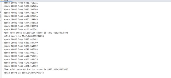
if __name__ == '__main__':
lr = lr_model()
data = lr.prepare_data()
for train, validation in lr.linear_cross_validation(data, 5):
X_train = train[:, :10]
y_train = train[:, -1].reshape((-1, 1))
X_valid = validation[:, :10]
y_valid = validation[:, -1].reshape((-1, 1))
loss5 = []
loss, params, grads = lr.linear_train(X_train, y_train, 0.001, 100000)
loss5.append(loss)
score = np.mean(loss5)
print('five kold cross validation score is', score)
y_pred = lr.predict(X_valid, params)
valid_score = np.sum(((y_pred - y_valid) ** 2)) / len(X_valid)
print('valid score is', valid_score)
逻辑回归
- 其实是分类算法

对应代码简易实现:

import numpy as np
import matplotlib.pyplot as plt
from sklearn.datasets import make_classification
class logistic_regression():
def __init__(self):
pass
def sigmoid(self, x):
z = 1 / (1 + np.exp(-x))
return z
def initialize_params(self, dims):
W = np.zeros((dims, 1))
b = 0
return W, b
def logistic(self, X, y, W, b):
num_train = X.shape[0]
num_feature = X.shape[1]
a = self.sigmoid(np.dot(X, W) + b)
cost = -1 / num_train * np.sum(y * np.log(a) + (1 - y) * np.log(1 - a))
dW = np.dot(X.T, (a - y)) / num_train
db = np.sum(a - y) / num_train
cost = np.squeeze(cost)
return a, cost, dW, db
def logistic_train(self, X, y, learning_rate, epochs):
W, b = self.initialize_params(X.shape[1])
cost_list = []
for i in range(epochs):
a, cost, dW, db = self.logistic(X, y, W, b)
W = W - learning_rate * dW
b = b - learning_rate * db
if i % 100 == 0:
cost_list.append(cost)
if i % 100 == 0:
print('epoch %d cost %f' % (i, cost))
params = {
'W': W,
'b': b
}
grads = {
'dW': dW,
'db': db
}
return cost_list, params, grads
def predict(self, X, params):
y_prediction = self.sigmoid(np.dot(X, params['W']) + params['b'])
for i in range(len(y_prediction)):
if y_prediction[i] > 0.5:
y_prediction[i] = 1
else:
y_prediction[i] = 0
return y_prediction
def accuracy(self, y_test, y_pred):
correct_count = 0
for i in range(len(y_test)):
for j in range(len(y_pred)):
if y_test[i] == y_pred[j] and i == j:
correct_count += 1
accuracy_score = correct_count / len(y_test)
return accuracy_score
def create_data(self):
X, labels = make_classification(n_samples=100, n_features=2, n_redundant=0, n_informative=2, random_state=1,
n_clusters_per_class=2)
labels = labels.reshape((-1, 1))
offset = int(X.shape[0] * 0.9)
X_train, y_train = X[:offset], labels[:offset]
X_test, y_test = X[offset:], labels[offset:]
return X_train, y_train, X_test, y_test
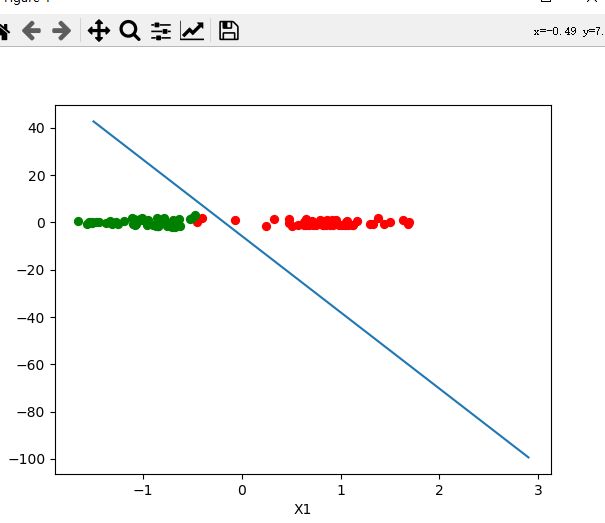
def plot_logistic(self, X_train, y_train, params):
n = X_train.shape[0]
xcord1 = []
ycord1 = []
xcord2 = []
ycord2 = []
for i in range(n):
if y_train[i] == 1:
xcord1.append(X_train[i][0])
ycord1.append(X_train[i][1])
else:
xcord2.append(X_train[i][0])
ycord2.append(X_train[i][1])
fig = plt.figure()
ax = fig.add_subplot(111)
ax.scatter(xcord1, ycord1, s=32, c='red')
ax.scatter(xcord2, ycord2, s=32, c='green')
x = np.arange(-1.5, 3, 0.1)
y = (-params['b'] - params['W'][0] * x) / params['W'][1]
ax.plot(x, y)
plt.xlabel('X1')
plt.ylabel('X2')
plt.show()
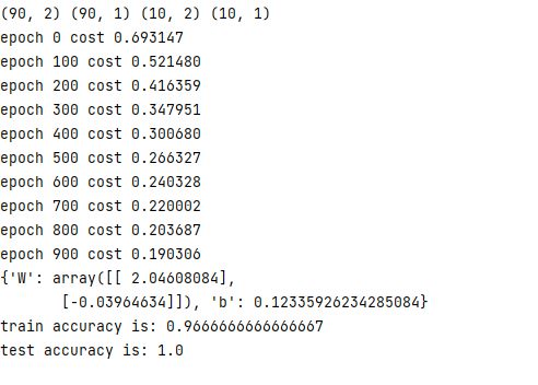
if __name__ == "__main__":
model = logistic_regression()
X_train, y_train, X_test, y_test = model.create_data()
print(X_train.shape, y_train.shape, X_test.shape, y_test.shape)
cost_list, params, grads = model.logistic_train(X_train, y_train, 0.01, 1000)
print(params)
y_train_pred = model.predict(X_train, params)
accuracy_score_train = model.accuracy(y_train, y_train_pred)
print('train accuracy is:', accuracy_score_train)
y_test_pred = model.predict(X_test, params)
accuracy_score_test = model.accuracy(y_test, y_test_pred)
print('test accuracy is:', accuracy_score_test)
model.plot_logistic(X_train, y_train, params)
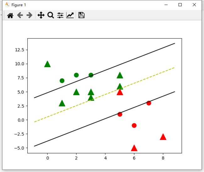
支持向量机
支持向量机是有监督学习中最具有影响力的方法之一,是基于线性判别函数的一种模型。
SVM基本思想:对于线性可分的数据,能将训练样本划分开的超平 面有很多,于是我们寻找“位于两类训练样本正中心的超平面”, 即margin最大化。从直观上看,这种划分对训练样本局部扰动的承 受性最好。事实上,这种划分的性能也表现较好。
一个判别面,两个支持向量,让判别面与支持向量的间隔最大。

遇事不决就加核

针对多类别的数据集或者复杂问题需要升维。
常用的核函数:
- 线性核
- 多项式核
- 高斯核(常用)
- 拉普拉斯核
- sigmoid 核
代码实现如下:
import numpy as np
import matplotlib.pyplot as plt

class Hard_Margin_SVM:
    def __init__(self, visualization=True):
        self.visualization = visualization
        self.colors = {
     1: 'r', -1: 'g'}
        if self.visualization:
            self.fig = plt.figure()
            self.ax = self.fig.add_subplot(1, 1, 1)

    # 定义训练函数
    def train(self, data):
        self.data = data
        # 参数字典 { ||w||: [w,b] }
        opt_dict = {
     }

        # 数据转换列表
        transforms = [[1, 1],
                      [-1, 1],
                      [-1, -1],
                      [1, -1]]

        # 从字典中获取所有数据
        all_data = []
        for yi in self.data:
            for featureset in self.data[yi]:
                for feature in featureset:
                    all_data.append(feature)

        # 获取数据最大最小值
        self.max_feature_value = max(all_data)
        self.min_feature_value = min(all_data)
        all_data = None

        # 定义一个学习率(步长)列表
        step_sizes = [self.max_feature_value * 0.1,
                      self.max_feature_value * 0.01,
                      self.max_feature_value * 0.001
                      ]

        # 参数b的范围设置
        b_range_multiple = 2
        b_multiple = 5
        latest_optimum = self.max_feature_value * 10

        # 基于不同步长训练优化
        for step in step_sizes:
            w = np.array([latest_optimum, latest_optimum])
            # 凸优化
            optimized = False
            while not optimized:
                for b in np.arange(-1 * (self.max_feature_value * b_range_multiple),
                                   self.max_feature_value * b_range_multiple,
                                   step * b_multiple):
                    for transformation in transforms:
                        w_t = w * transformation
                        found_option = True

                        for i in self.data:
                            for xi in self.data[i]:
                                yi = i
                                if not yi * (np.dot(w_t, xi) + b) >= 1:
                                    found_option = False
                                    # print(xi,':',yi*(np.dot(w_t,xi)+b))

                        if found_option:
                            opt_dict[np.linalg.norm(w_t)] = [w_t, b]

                if w[0] < 0:
                    optimized = True
                    print('Optimized a step!')
                else:
                    w = w - step

            norms = sorted([n for n in opt_dict])
            # ||w|| : [w,b]
            opt_choice = opt_dict[norms[0]]
            self.w = opt_choice[0]
            self.b = opt_choice[1]
            latest_optimum = opt_choice[0][0] + step * 2

        for i in self.data:
            for xi in self.data[i]:
                yi = i
                print(xi, ':', yi * (np.dot(self.w, xi) + self.b))

                # 定义预测函数

    def predict(self, features):
        # sign( x.w+b )
        classification = np.sign(np.dot(np.array(features), self.w) + self.b)
        if classification != 0 and self.visualization:
            self.ax.scatter(features[0], features[1], s=200, marker='^', c=self.colors[classification])
        return classification

    # 定义结果绘图函数
    def visualize(self):
        [[self.ax.scatter(x[0], x[1], s=100, color=self.colors[i]) for x in data_dict[i]] for i in data_dict]

        # hyperplane = x.w+b
        # v = x.w+b
        # psv = 1
        # nsv = -1
        # dec = 0
        # 定义线性超平面
        def hyperplane(x, w, b, v):
            return (-w[0] * x - b + v) / w[1]

        datarange = (self.min_feature_value * 0.9, self.max_feature_value * 1.1)
        hyp_x_min = datarange[0]
        hyp_x_max = datarange[1]

        # (w.x+b) = 1
        # 正支持向量
        psv1 = hyperplane(hyp_x_min, self.w, self.b, 1)
        psv2 = hyperplane(hyp_x_max, self.w, self.b, 1)
        self.ax.plot([hyp_x_min, hyp_x_max], [psv1, psv2], 'k')

        # (w.x+b) = -1
        # 负支持向量
        nsv1 = hyperplane(hyp_x_min, self.w, self.b, -1)
        nsv2 = hyperplane(hyp_x_max, self.w, self.b, -1)
        self.ax.plot([hyp_x_min, hyp_x_max], [nsv1, nsv2], 'k')

        # (w.x+b) = 0
        # 线性分隔超平面
        db1 = hyperplane(hyp_x_min, self.w, self.b, 0)
        db2 = hyperplane(hyp_x_max, self.w, self.b, 0)
        self.ax.plot([hyp_x_min, hyp_x_max], [db1, db2], 'y--')

        plt.show()


data_dict = {
     -1: np.array([[1, 7],
                           [2, 8],
                           [3, 8], ]),

             1: np.array([[5, 1],
                          [6, -1],
                          [7, 3], ])}

if __name__ == '__main__':

    svm = Hard_Margin_SVM()
    svm.train(data=data_dict)

    predict_us = [[0, 10],
                  [1, 3],
                  [3, 4],
                  [3, 5],
                  [5, 5],
                  [5, 6],
                  [6, -5],
                  [5, 8],
                  [2, 5],
                  [8, -3]]

    for p in predict_us:
        svm.predict(p)

    svm.visualize()

决策树
这里主要涉及到熵的概念、相关请往上面复习:
熵,条件熵,信息增益、基尼指数。
决策树是一种基于树结构进行决策的机器学习方法,这恰是人类面临决策 时一种很自然的处理机制。
在这些树的结构里,叶子节点给出类标而内部节点代表某个属性;
例如,银行在面对是否借贷给客户的问题时,通常会进行一系列的决 策。银行会首先判断:客户的信贷声誉是否良好?良好的话,再判断 客户是否有稳定的工作? 不良好的话,可能直接拒绝,也可能判断客 户是否有可抵押物?..这种思考过程便是决策树的生成过程。
决策树的生成过程中,最重要的因素便是根节点的选择,即选择哪种特征作为决策因素:ID3算法使用信息增益作为准则。
import numpy as np
import pandas as pd
from math import log

df = pd.read_csv('./example_data.csv')
def entropy(ele):
    '''
    function: Calculating entropy value.
    input: A list contain categorical value.
    output: Entropy value.
    entropy = - sum(p * log(p)), p is a prob value.
    '''
    # Calculating the probability distribution of list value
    probs = [ele.count(i)/len(ele) for i in set(ele)]
    # Calculating entropy value
    entropy = -sum([prob*log(prob, 2) for prob in probs])
    return entropy
def split_dataframe(data, col):
    '''
    function: split pandas dataframe to sub-df based on data and column.
    input: dataframe, column name.
    output: a dict of splited dataframe.
    '''
    # unique value of column
    unique_values = data[col].unique()
    # empty dict of dataframe
    result_dict = {
     elem : pd.DataFrame for elem in unique_values}
    # split dataframe based on column value
    for key in result_dict.keys():
        result_dict[key] = data[:][data[col] == key]
    return result_dict
 class ID3Tree:
    # define a Node class
    class Node:
        def __init__(self, name):
            self.name = name
            self.connections = {
     }

        def connect(self, label, node):
            self.connections[label] = node

    def __init__(self, data, label):
        self.columns = data.columns
        self.data = data
        self.label = label
        self.root = self.Node("Root")

    # print tree method
    def print_tree(self, node, tabs):
        print(tabs + node.name)
        for connection, child_node in node.connections.items():
            print(tabs + "\t" + "(" + connection + ")")
            self.print_tree(child_node, tabs + "\t\t")

    def construct_tree(self):
        self.construct(self.root, "", self.data, self.columns)

    # construct tree
    def construct(self, parent_node, parent_connection_label, input_data, columns):
        max_value, best_col, max_splited = choose_best_col(input_data[columns], self.label)
        if not best_col:
            node = self.Node(input_data[self.label].iloc[0])
            parent_node.connect(parent_connection_label, node)
        return

        node = self.Node(best_col)
        parent_node.connect(parent_connection_label, node)

        new_columns = [col for col in columns if col != best_col]
        # Recursively constructing decision trees
        for splited_value, splited_data in max_splited.items():
            self.construct(node, splited_value, splited_data, new_columns)
from sklearn.datasets import load_iris
from sklearn import tree
import graphviz

iris = load_iris()
# criterion选择entropy,这里表示选择ID3算法
clf = tree.DecisionTreeClassifier(criterion='entropy', splitter='best')
clf = clf.fit(iris.data, iris.target)

dot_data = tree.export_graphviz(clf, out_file=None,
                               feature_names=iris.feature_names,
                               class_names=iris.target_names,
                               filled=True,
                               rounded=True,
                               special_characters=True)
graph = graphviz.Source(dot_data)
随机森林
树桩算法
无监督学习
数据集没有标记信息(自学)
- 聚类:我们可以使用无监督学习来预测各样本之间的关联度,把关 联度大的样本划为同一类,关联度小的样本划为不同类,这便是 “聚类”
- 降维:我们也可以使用无监督学习处理数据,把维度较高、计算复 杂的数据,转化为维度低、易处理、且蕴含的信息不丢失或较少丢 失的数据,这便是“降维”
聚类
聚类的目的是将数据分成多个类别,在同一个类内,对象(实体)之间具 有较高的相似性,在不同类内,对象之间具有较大的差异。
对一批没有类别标签的样本集,按照样本之间的相似程度分类,相似的归为一类,不相似的归为其它类。这种分类称为聚类分析,也 称为无监督分类
常见方法有K-Means聚类、均值漂移聚类、基于密度的聚类等。
kmeans

-
选取数据空间中的K个对象作为初始中心,每个对象代表一个聚 类中心;
-
对于样本中的数据对象,根据它们与这些聚类中心的欧氏距离, 按距离最近的准则将它们分到距离它们最近的聚类中心(最相似) 所对应的类;
-
更新聚类中心:将每个类别中所有对象所对应的均值作为该类别 的聚类中心,计算目标函数的值;
-
判断聚类中心和目标函数的值是否发生改变,若不变,则输出结 果,若改变,则返回2)。
注意:
聚类的结果会受到 初始随机选的中心点分布 + 数据分布影响
在一堆数据点中随机位置生成两个中心点,算得数据点距离两个中心点的距离,归为距离短的一类—>一类的所有距离算均值,然后通过距离均值在对应位置重新生成中心点,继续算新中心点的距离,归为距离短的一类—>步骤重复 -
kmeas 有个init,随机选取最远的点进行聚类,效果更加,kmeans++
均值漂移(不需要指定聚类数)
生产一个中心点,以其为圆心作圆算这个点到所有点的向量平均值,若园内密度大且分布均匀则结束,反之移动圆心寻找新的位置

层次聚类
逐层聚类;注意聚类的程度,避免过拟合,聚类成只有一个类了
- 最短距离法、最长距离法、中间距离法
- 最短:由小到大,聚少成多
- 最长:从总得开始,一层一层分剥
- 中间:取中间距离为分界线用来聚类

- 用树来聚类,很容易过了,过了!!!!
密度聚类
密度聚类 图里minpts = 3 (可能会出现离群点)
领域:例 x1为圆心,圆范围内就是领域

密度直达—一定要在领域之内
密度可达----x1的密度直达x2有个密度直达x3,那么x1的密度可达就是x3
密度相连:x3和x4密度相连
- 不需要指定k
- 需要指定圈大小/圈内节点数
- 计算慢
容易出现离群点。
混合高斯聚类
混合高斯(算出分布拟合,然后聚类)
拟合出两个高斯分布之后,数据点在两个高斯分布里做比较
EM算法(最大期望算法)
- 求P(A、B):固定数据B,P(A|B)---->反顾来固定求得的A,
- P(B|A)---->继续P(A|B),不停迭代打到精确值
AP(近邻传播算法affinity propagation )聚类
吸引信息:一种矩阵,类似表现自身的相似性
归属信息:一种矩阵,类似用自身比较吸引信息的相似性
降维
降维的目的就是将原始样本数据的维度降低到一个更小的数,且尽量使得样本蕴含信息量损失最小,或还原数据时产生的误差最小。比如主成分分析法…
- 数据在低维下更容易处理、更容易使用;
- 相关特征,特别是重要特征更能在数据中明确的显示出来;
- 如果只有二维或者三维的话,能够进行可视化展示;
- 去除数据噪声,降低算法开销等。
PCA主成分分析(无监督)
- 对特征作分解(旋转基),影响小/无影响的特征分向量可以取掉
特征之间做协方差矩阵,将矩阵做对角化,然后矩阵中影响小的特征值去掉
有时候,特征之间不是完全的独立,彼此会有些影响,需要作降维处理,去掉关系
降维目的:相同特征之间方差越大越好;不同特征之间方差越小越好

LDA 线性判别分析,有监督降维,也可做分类
-其实就是,在k-1维空间找一个判别面。
参考:
链接: 机器学习
链接: DataWhale.