pytorch实现lstm分类模型

教程原文在这里Tutorial，这篇文章中用LSTM实现了一个简单的词类标注模型。下面是一些具体的解析：

# Author: Robert Guthrie

import torch
import torch.nn as nn
import torch.nn.functional as F
import torch.optim as optim

torch.manual_seed(1)
# 引用库函数

我们首先了解如何初始化一个nn.LSTM实例， 以及它的输入输出。初始化nn.LSTM实例， 可以设定的参数如下：

常用的是前两个，用来描述LSTM输入的词向量维度和输出的向量的维度（与hidden state相同），其中num_layer指的是这样的结构：

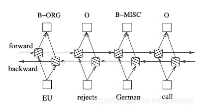
这种称作stacked LSTM，如上就是两层LSTM堆叠起来。bi-direction指的是双向，双向的LSTM会从正反两个方向读句子，依次输入词向量， 两个方向的hidden state也并不是公共的，如下图：

对应到下面代码的第一行，就是创建了一个输入输出的维度均为3、单层单向的LSTM网络。

lstm = nn.LSTM(3, 3)  # Input dim is 3, output dim is 3
inputs = [torch.randn(1, 3) for _ in range(5)]  # make a sequence of length 5

这个网络的输入输出怎么样呢？LSTM的基本功能是接收一个句子（一个词向量序列），从第一个词开始逐个后移，移到每一个词的时候，根据hidden state、cell state以及当前的词向量计算输出，并更新hidden state 和cell state，因此输入首先是一个词向量列，同时也可以设定一开始的hidden state和cell state，如果不设定那就自动初始化为0。而输出有三个，一个是每一步的输出构成的序列，这里每一个输出对应句子中的每一个词，第二个输出是最后的hidden state，第三个则是最后的cell state，具体的输入输出如下图：

# initialize the hidden state.
hidden = (torch.randn(1, 1, 3),
          torch.randn(1, 1, 3))
          
for i in inputs:
    # Step through the sequence one element at a time.
    # after each step, hidden contains the hidden state.
    out, hidden = lstm(i.view(1, 1, -1), hidden)

# alternatively, we can do the entire sequence all at once.
# the first value returned by LSTM is all of the hidden states throughout
# the sequence. the second is just the most recent hidden state
# (compare the last slice of "out" with "hidden" below, they are the same)
# The reason for this is that:
# "out" will give you access to all hidden states in the sequence
# "hidden" will allow you to continue the sequence and backpropagate,
# by passing it as an argument  to the lstm at a later time
# Add the extra 2nd dimension
inputs = torch.cat(inputs).view(len(inputs), 1, -1)
hidden = (torch.randn(1, 1, 3), torch.randn(1, 1, 3))  # clean out hidden state
out, hidden = lstm(inputs, hidden)
print(out)
print(hidden)

如上，hidden实际上是(h0, c0)，它的三个维度的含义是(num_layer*num_direction, batch_size, hidden_size)，第一维和第三维都是由LSTM实例的参数确定的，batch_size倒是很特别，如果hidden的第二个维度不为1，那难道不同的batch的hidden state不会公用吗？
LSTM的输入维度也很有意思，三个维度的含义为：（sequence_len, batch_size, input_size），第三个维度就是词向量embedding长度，sequence len是句长，batch_size是分批的大小，这跟我们一般常用表示方式(batch_size, sequence_len, input_size) 相反。而且我们看到使用时总是配合tensor.view这个方法， 这个方法其实就是tensor的reshape， 它究竟会让tensor怎样重新排列呢？我们可以看下面的结果：

	input = np.array([11, 12, 21, 22, 31, 32])
    input_tensor = torch.from_numpy(input)
    print(input_tensor.view(2, 3, 1))

输出：

tensor([[[11],
         [12],
         [21]],

        [[22],
         [31],
         [32]]])

按照LSTM的理解，这样的input就是3个长为2的句子为一批，每一个词向量维度都是1。我们的第一个句子是[11, 22]，第二个是[12, 31]，这就有一个问题，原本是连续输入的单词，现在反而被隔开了，假设我们的输入数据是一句话连着一句话，LSTM反而会理解为每一个句子的开头连成一句话。比如上面，LSTM神经网络就是先输入i = [[11], [12], [21]]，这三者没有先后顺序，而是平行地进行向量运算：
（联想到刚刚h的维度是(batch_size, hidden_size)(不考虑双向和stack)，更加可以说明这里batch中各个矩阵运算其实就是平行的）

然后再输入每句话的第二个词[[22], [31], [32]]这时，会分别利用到前面三个的hidden state、cell state并且更新。
其实我觉得这样设计还挺迷的，如果要保持原句的样式，输入的时候是不是要把句子拆开，把同一批的开头放在一起、第二个词放在一起···
接下来正式开始词类标注标注的模型实例。我们实际上训练时可以这样做：先将输入向量拆分成batch x sentence x embedding这样的常规形式，也就是tensor = tensor.view(-1, sentence_len, input_size)，这样分批时就可以直接将batch=tensor(i*batch_size: (i+1)*batch_size, :, :)送进LSTM，送进LSTM时对前两维做一个转置就好了：output = LSTM(batch.transpose(0, 1))，这样做还保证了连续性（contiguous）。
其实除了batch之外也没什么好说的，而这个实例的batch恰好是1‍♀️：

def prepare_sequence(seq, to_ix):
    idxs = [to_ix[w] for w in seq]
    return torch.tensor(idxs, dtype=torch.long)


training_data = [
    ("The dog ate the apple".split(), ["DET", "NN", "V", "DET", "NN"]),
    ("Everybody read that book".split(), ["NN", "V", "DET", "NN"])
]
word_to_ix = {}
for sent, tags in training_data:
    for word in sent:
        if word not in word_to_ix:
            word_to_ix[word] = len(word_to_ix)
print(word_to_ix)
tag_to_ix = {"DET": 0, "NN": 1, "V": 2}

# These will usually be more like 32 or 64 dimensional.
# We will keep them small, so we can see how the weights change as we train.
EMBEDDING_DIM = 6
HIDDEN_DIM = 6

上面就是把每个单词编了号，用数字代表单词，当然这个数字不能直接用于训练，还需要embedding（不过这个embedding也没啥，毕竟总共才两句话）
输出：

{'The': 0, 'dog': 1, 'ate': 2, 'the': 3, 'apple': 4, 'Everybody': 5, 'read': 6, 'that': 7, 'book': 8}

接下来我们用nn.LSTM和全连接神经网络层nn.Linear来搭建我们的神经网络模型：

class LSTMTagger(nn.Module):

    def __init__(self, embedding_dim, hidden_dim, vocab_size, tagset_size):
        super(LSTMTagger, self).__init__()
        self.hidden_dim = hidden_dim

        self.word_embeddings = nn.Embedding(vocab_size, embedding_dim)

        # The LSTM takes word embeddings as inputs, and outputs hidden states
        # with dimensionality hidden_dim.
        self.lstm = nn.LSTM(embedding_dim, hidden_dim)

        # The linear layer that maps from hidden state space to tag space
        self.hidden2tag = nn.Linear(hidden_dim, tagset_size)

    def forward(self, sentence):
        embeds = self.word_embeddings(sentence)
        lstm_out, _ = self.lstm(embeds.view(len(sentence), 1, -1))
        tag_space = self.hidden2tag(lstm_out.view(len(sentence), -1))
        tag_scores = F.log_softmax(tag_space, dim=1)
        return tag_scores

vocab_size 指的是我们的词库大小，两句话总共8个词所以是8。target_size是我们自己定义的输出维度，我们的LSTM不直接输出，而是经过一个全连接神经网络之后再输出，这个过程可以改变维度。由于是词类标注，其实就是多分类任务，我们输出的维度和可能的分类数量一样，输出每一个维度可以理解为此分类的得分score，得分越高就代表此分类是正确分类的可能性越大。

model = LSTMTagger(EMBEDDING_DIM, HIDDEN_DIM, len(word_to_ix), len(tag_to_ix))
loss_function = nn.NLLLoss()
optimizer = optim.SGD(model.parameters(), lr=0.1)

# See what the scores are before training
# Note that element i,j of the output is the score for tag j for word i.
# Here we don't need to train, so the code is wrapped in torch.no_grad()
with torch.no_grad():
    inputs = prepare_sequence(training_data[0][0], word_to_ix)
    tag_scores = model(inputs)
    print(tag_scores)
## 这里只是用完全没训练过的LSTM来预测一下。

for epoch in range(300):  # again, normally you would NOT do 300 epochs, it is toy data
    for sentence, tags in training_data:
        # Step 1. Remember that Pytorch accumulates gradients.
        # We need to clear them out before each instance
        model.zero_grad()

        # Step 2. Get our inputs ready for the network, that is, turn them into
        # Tensors of word indices.
        sentence_in = prepare_sequence(sentence, word_to_ix)
        targets = prepare_sequence(tags, tag_to_ix)

        # Step 3. Run our forward pass.
        tag_scores = model(sentence_in)

        # Step 4. Compute the loss, gradients, and update the parameters by
        #  calling optimizer.step()
        loss = loss_function(tag_scores, targets)
        loss.backward()
        optimizer.step()

# See what the scores are after training
with torch.no_grad():
    inputs = prepare_sequence(training_data[0][0], word_to_ix)
    tag_scores = model(inputs)

    # The sentence is "the dog ate the apple".  i,j corresponds to score for tag j
    # for word i. The predicted tag is the maximum scoring tag.
    # Here, we can see the predicted sequence below is 0 1 2 0 1
    # since 0 is index of the maximum value of row 1,
    # 1 is the index of maximum value of row 2, etc.
    # Which is DET NOUN VERB DET NOUN, the correct sequence!
    print(tag_scores)

上面的loss function是nn.NLLLoss，这是一个多分类误差函数类，每一个实例的输入输出如下：

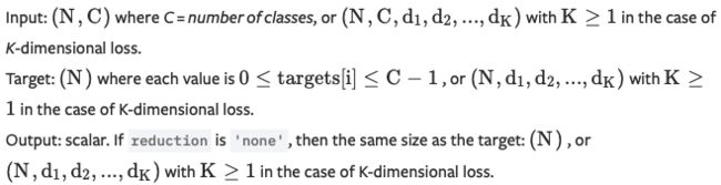
input是N个长为C的向量，代表一批中的N个实例在C个标签下的打分，而target是这N个标签的正确分类。