TensorFlow2.0入门到进阶2.9 —— 实战深度神经网络

1、写在前面

有人会问，2.88在哪呢？其实2.8是一些基础理论知识，这一部分在2.1已经介绍的很详细了，如果不了解看看2.1吧。

这里说个知识点吧：

• dropout

通俗来说，就是将训练好的十分复杂的神经网络，去除一部分连接，如下图所示。那么有人会问，这么费劲训练好的网络，为什么还要去掉一部分连接？这主要是为了提高训练模型的泛化能力。

一般在深度神经网络中应用，由于层数较深，容易出现过拟合，这时候在倒数第一、二层之间通常将如dropout。

详见：https://www.cnblogs.com/fpzs/p/9715044.html

2、深度神经网络

前几节已经讲了神经网络，那何为深度神经网络，通俗来说就是层数很多的神经网络，有什么优点能？如果数据量足够多的话，他所发现的特征会更多，相对来说准确率会更高。下面通过一个20层网络的例子来说明。

3、举个栗子

大体程序和之前那个服装分类的例子一样，如果不了解的小伙伴，看一下：一个服装分类项目轻松入门TensorFlow

import matplotlib as mpl
import matplotlib.pyplot as plt
#为了在jupyter notebook中画图
%matplotlib inline
import numpy as np
import sklearn
import pandas as pd
import os
import sys
import time
import tensorflow as tf
from tensorflow import keras

print(tf.__version__)
print(sys.version_info)
for module in mpl,np,pd,sklearn,tf,keras:
    print(module.__name__,module.__version__)
    
fashion_mnist=keras.datasets.fashion_mnist
(x_train_all,y_train_all),(x_test,y_test)=fashion_mnist.load_data()
x_valid,x_train=x_train_all[:5000],x_train_all[5000:]
y_valid,y_train=y_train_all[:5000],y_train_all[5000:]

print(x_valid.shape,y_valid.shape)
print(x_train.shape,y_train.shape)
print(x_test.shape,y_test.shape)

# x=(x-u)/std   符合正态分布

from sklearn.preprocessing import StandardScaler
#之前x_train为np.int型，所以先转为float32
#fit_transform()为归一化函数，要求输入为一维数组，并将记录均值和方差
#transform()为归一化函数，但不记录均值和方差，使用之前的均值和方差
#reshape(-1,1)表示将原数据转为n行1列的数组，-1根据原数组的数据量决定

scaler = StandardScaler()
x_train_scaled = scaler.fit_transform(
    x_train.astype(np.float32).reshape(-1,1)).reshape(-1,28,28)
x_valid_scaled = scaler.transform(
    x_valid.astype(np.float32).reshape(-1,1)).reshape(-1,28,28)
x_test_scaled = scaler.transform(
    x_test.astype(np.float32).reshape(-1,1)).reshape(-1,28,28)

下面创建网络的方式和之前一样，只不过中间通过一个循环，加入了20层，如果数据足够大的话，可以考虑加入更多层，但是如果数据小，可能出现过拟合。

model=keras.models.Sequential()
#添加输入层，输入的图片展开，Flatten为展平
model.add(keras.layers.Flatten(input_shape=[28,28]))

# 层数达到足够大时构成深度神经网络 DNN
for  _i in range(20):
    model.add(keras.layers.Dense(100,activation='relu'))
model.add(keras.layers.Dense(10,activation='softmax'))

model.compile(loss='sparse_categorical_crossentropy',
              optimizer='adam',
              metrics=['accuracy'])

下面具体看一下创建的神经网络：

model.summary()

Model: "sequential_1"
_________________________________________________________________
Layer (type)                 Output Shape              Param #   
=================================================================
flatten_1 (Flatten)          (None, 784)               0         
_________________________________________________________________
dense_21 (Dense)             (None, 100)               78500     
_________________________________________________________________
dense_22 (Dense)             (None, 100)               10100     
_________________________________________________________________
dense_23 (Dense)             (None, 100)               10100     
_________________________________________________________________
dense_24 (Dense)             (None, 100)               10100     
_________________________________________________________________
dense_25 (Dense)             (None, 100)               10100     
_________________________________________________________________
dense_26 (Dense)             (None, 100)               10100     
_________________________________________________________________
dense_27 (Dense)             (None, 100)               10100     
_________________________________________________________________
dense_28 (Dense)             (None, 100)               10100     
_________________________________________________________________
dense_29 (Dense)             (None, 100)               10100     
_________________________________________________________________
dense_30 (Dense)             (None, 100)               10100     
_________________________________________________________________
dense_31 (Dense)             (None, 100)               10100     
_________________________________________________________________
dense_32 (Dense)             (None, 100)               10100     
_________________________________________________________________
dense_33 (Dense)             (None, 100)               10100     
_________________________________________________________________
dense_34 (Dense)             (None, 100)               10100     
_________________________________________________________________
dense_35 (Dense)             (None, 100)               10100     
_________________________________________________________________
dense_36 (Dense)             (None, 100)               10100     
_________________________________________________________________
dense_37 (Dense)             (None, 100)               10100     
_________________________________________________________________
dense_38 (Dense)             (None, 100)               10100     
_________________________________________________________________
dense_39 (Dense)             (None, 100)               10100     
_________________________________________________________________
dense_40 (Dense)             (None, 100)               10100     
_________________________________________________________________
dense_41 (Dense)             (None, 10)                1010      
=================================================================
Total params: 271,410
Trainable params: 271,410
Non-trainable params: 0

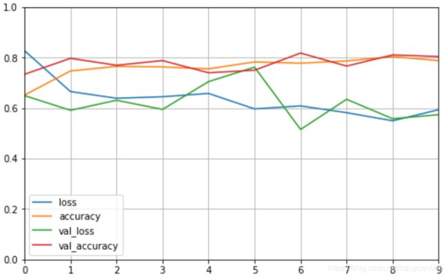
观察一下训练结果：

def plot_learning_curves(history):
    #设置画布大小为8和5
    pd.DataFrame(history.history).plot(figsize=(8,5))
    #显示网格
    plt.grid(True)
    #set_ylim为设置y坐标轴的范围
    plt.gca().set_ylim(0,1)
    plt.show()
    
plot_learning_curves(history)

#初期，目标函数基本不变，之后发生变化陡峭原因：
#1、模型较深，参数众多，训练不充分
#2、梯度消失 ->深度神经网络中 链式法则  ->复合函数f(g(x))