1. Conditional probability

2. Bayes theorem

P(A | B) is a conditional probability: the likelihood of event A occurring given that B is true.
P(B | A) is also a conditional probability: the likelihood of event B occurring given that A is true.
P(A) and P(B) are the probabilities of observing A and B independently of each other; this is known as the marginal probability.
Bayes theorem Interpretations:
Bayesian inference derives the posterior probability as a consequence of two antecedents: a prior probability and a "likelihood function" derived from a statistical model for the observed data. Bayesian inference computes the posterior probability according to Bayes' theorem:

H: stands for any hypothesis whose probability may be affected by data (called evidence below). Often there are competing hypotheses, and the task is to determine which is the most probable.
P(H): the prior probability, is the estimate of the probability of the hypothesis H before the data E, the current evidence, is observed.
P(H | E): the posterior probability, is the probability of H given E, i.e., after E is observed. This is what we want to know: the probability of a hypothesis given the observed evidence.
P(E | H): is the probability of observing E given H, and is called the likelihood. As a function of E with H fixed, it indicates the compatibility of the evidence with the given hypothesis. The likelihood function is a function of the evidence, E, while the posterior probability is a function of the hypothesis, H.
P(E): is sometimes termed the marginal likelihood or "model evidence". This factor is the same for all possible hypotheses being considered (as is evident from the fact that the hypothesis H does not appear anywhere in the symbol, unlike for all the other factors), so this factor does not enter into determining the relative probabilities of different hypotheses.
For different values of H, only the factors P(H) and P(E | H), both in the numerator, affect the value of P(H | E) – the posterior probability of a hypothesis is proportional to its prior probability (its inherent likeliness) and the newly acquired likelihood (its compatibility with the new observed evidence).
Sometimes, Bayes theorem can be written as:

where the factor P(E | H) / P(E) can be interpreted as the impact of E on the probability of H.
3. Binomial distribution
Binomial distribution with parameters n and p is the discrete probability distribution of the number of successes in a sequence of n independent experiments, each asking a yes–no question, and each with its own Boolean-valued outcome: a random variable containing a single bit of information: success/yes/true/one (with probability p) or failure/no/false/zero (with probability q = 1 − p).
In general, if the random variable X follows the binomial distribution with parameters n ∈ ℕ and p ∈ [0,1], we write X ~ B(n, p). The probability of getting exactly k successes in n trials is given by the probability mass function:


The cumulative distribution function can be expressed as:

Mean: E(X) = np; Variance: Var(X) = npq = np(1-q); Mode:

*Covariance between two binomials:
If two binomially distributed random variables X and Y are observed together, estimating their covariance can be useful. The covariance is Cov(X,Y) = E(XY) - μX * μY
In the case n= 1 (the case of Bernoulli trials) XY is non-zero only when both X and Y are one, and μX and μY are equal to the two probabilities. Defining pB as the probability of both happening at the same time, this gives
In a bivariate setting involving random variables X and Y, there is a particular expectation that is often of interest. It is called covariance and is given by: Cov(X,Y) = E((X-E(X))(Y-E(Y)) where the expectation is taken over the bivariate distribution of X and Y. Alternatively, Cov(X,Y) = E(XY) - E(X)E(Y)
Moreover, a scaled version of covariance is the correlation ρ which is given by
ρ = Corr(X,Y) = Cov(x,y) / [sqrt(Var(X)*sqrt(Var(Y)], Var(X)=σx^2
The correlation ρ is the population analogue of the sample correlation coefficient r that is used to describe the degree of linear relationship involving paired data.
Confidence Interval
Assume that total number of successes X ~ B(n,p) with np>=5, n(1-p)>=5 so that the normal approximation to the binomial is reasonable.
In practice, p is unknown. Under the normal approximation, we have X ~ N(np, np(1-p)) and we define p^ = X/n as the proportion of successes. Since p^ is a linear combination of normal random variable, it follows that p^ ~ N(p,p(1-p)/n) then the probability statement is

Let Za/2 denote the (1-a/2)100-th percentile for the standard normal distribution, a (1-a)100% approximation confidence interval (because we user normal distribution to the binomial and the substitution of p with p-hat) for p-hat is given by

4. Normal distribution
the normal (or Gaussian) distribution is a very common continuous probability distribution. Normal distributions are important in statistics and are often used in the natural and social sciences to represent real-valued random variables whose distributions are not known.
If X ~ N(μ,σ^2), then E(X) = μ, and Var(X) = σ^2
σ^2 is the variance and not the standard deviation.
A random variable Z ~ N(0,1) is referred to as standard normal and it has the simplified pdf:

The relationship between an arbitrary normal random variable X ~ N(μ, σ^2) and the standard normal distribution is expressed via (X-μ) / σ ~ N(0,1)
Confidence Interval
In this case, we assume X1,X2,...,XN iid normal(μ, σ^2) where our interest concerns that μ is unknown and σ is known for ease of development. (In real world, we can't find a case with known σ & unknown μ)
X-bar ~ N(μ, σ^2/n)
Rearranging terms:
Finally, we obtain a 95% confidence interval (as follows) for μ
More generally, let Za/2 denote the (1-a/2)100-th percentile for the standard normal distribution, a (1-a)100% confidence interval for μ is given by
we use the observed value x-bar. It is understood that confidence intervals are functions of observed statistics.
When n is large, it turns out that the sample standard deviation s provides a good estimate of σ. Therefore, we are able to to provide a confidence interval for μ in the more realistic case where σ is unknown. We simply replace σ in above mentioned functions with s.
5. Descriptive statistics
It concerns the presentation of data (either numerical or graphical) in a way that makes it easier to digest data.
Dotplot: for univariate data
outliers: too big or small
centrality: values in the middle portion of the dotplot
dispersion: spread or variation in the data
Histograms: for univariate data, the size of dataset n is fairly large
modality: a histogram with two distinct humps is referred to as bimodal
skewness:
symmetry:
How to choose interval as x-axis: choose the number of intervals roughly equal to sqrt(n) where n is the number of observations.
For those intervals are not equal length, we should plot relative frequency divided by intervals length on the vertical axis, instead of using frequency.
Boxplot: for univariate data, is most appropriately used when the data are divided into groups.
sample median (Q2); top-edge is 3/4 quantile (Q3); bottom-edge: 1/4 quantile (Q1)
interquartile range (IQR) : Q3-Q1, known as ΔQ
maximum interval: Q3+1.5ΔQ or 90th percentile
minimum interval: Q1-1.5ΔQ or 10th percentile
values that out of max & min intervals are Outliers.
whiskers (vertical dashed lines) extend to the outer limits of the data and circles correspond to outliers.
Scatterplot: it is appropriate for paired data
extrapolated data: when predicting, you should be cautious about predictions based on extrapolated data. There perhaps appears a positive increase trend from the pairplot with two variables X,Y, but it doesn't mean they have the same relationship for X, Y. (Data should be combined with the real world)
Correlation Coefficient: measure the degree of linear association between x and y
It is a numerical descriptive statistic for investigating paired data is the sample correlation or correlation or correlation coefficient r defined by

Properties:
-1 <= r <= 1
when r close to 1, the points are clustered about a line with positive slope
when r close to -1, the points are clustered about a line with negative slope
when r close to 0, points are lack of linear relationship. However, there may be a quadratic relationship
when x and y are correlated (not close to 0), it merely denotes the presence of a linear association. For example, weight and height are positively correlated, and it is obviously wrong to state that one causes the other.
In order to establish cause and effect relationship, we should do a controlled study.

6. Law of large numbers
the average of the results obtained from a large number of trials should be close to the expected value, and will tend to become closer as more trials are performed.
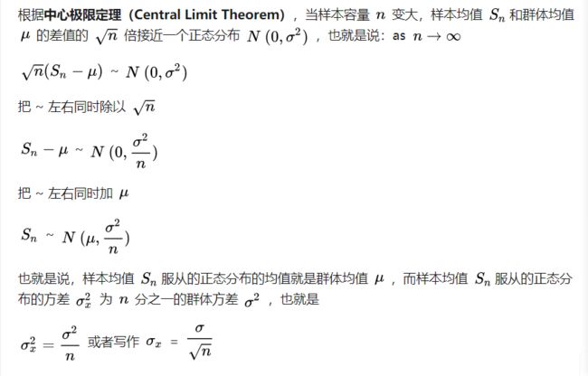
7. Central limited theorem
For the CLT, we assume that the random variables X1,X2,...,Xn are *iid from a population with mean μ and variance σ^2. The CLT states that as n => infinity, the distribution of *(X_bar - μ)/(σ/sqrt(n)) converges to the distribution of a standard normal random variable.
*iid: independent and identically distributed, which means X's are independent of one another and arise from the same probability distribution.
从一个均值为 μ 、标准差为σ的总体中选取一个有n个观测值的随机样本。那么当n足够大时,x¯的抽样分布将近似服从均值μx¯=μ、标准差σx¯=σ/√n的正态分布。并且样本量越大,对x¯的抽样分布的正太近似越好
In probability theory, the central limit theorem (CLT) establishes that, in some situations, when independent random variables are added, their properly normalized sum tends toward a normal distribution (informally a "bell curve") even if the original variables themselves are not normally distributed.
要求:
1. 总体本身的分布不要求正态分布
2. 样本每组要足够大,但也不需要太大 n≥30
中心极限定理在理论上保证了我们可以用只抽样一部分的方法,达到推测研究对象统计参数的目的。
8. Linear regression: not mentioned Gradient Descent and Cost Function in machine learning aspect.
linear regression is predicting the value of a variable Y(dependent variable) based on some variable X(independent variable) provided there is a linear relationship between X and Y.
Y=b0 + b1X+e
(Recall that the regression equation without the error term, Y=b0 + b1X , is called the least squares line.)


SSTO, a.k.a SST, sum of squared total: sum of difference from the mean of y and data point yi
SSE, sum of squared error: sum of difference from the estimated regression line and data point yi
SSR, sum of squared regression: quantifies how far the estimated sloped regression line, y^i, is from the horizontal "no relationship line," the sample mean or y¯.
SST = SSR + SSE
From the above example, it tells us that most of the variation in the response y (SSTO = 1827.6) is just due to random variation (SSE = 1708.5), not due to the regression of y on x (SSR = 119.1).
Coefficient of Determination or r^2

If r^2 = 1, all data points fall perfectly on the regression line. The predictor x accounts for all of the variation in y!
If r^2 = 0, the estimated regression line is perfectly horizontal. The predictor x accounts for none of the variation in y!
r^2 ×100 percent of the variation in y is 'explained by' the variation in predictor x.
SSE is the amount of variation that is left unexplained by the model.
R-squared Cautions:
1. The coefficient of determination r^2 and the correlation coefficient r quantify the strength of a linear relationship. It is possible that r^2 = 0% and r = 0, suggesting there is no linear relation between x and y, and yet a perfect curved (or "curvilinear" relationship) exists.
[Most misinterpreting concept] 2. A large r^2 value should not be interpreted as meaning that the estimated regression line fits the data well.

Although the R-squared value is 92% and only 8% of the variation US population is left to explain after taking into account the year in a linear way. The plot suggests that a curve plot describe the relationship even better. (Its large value does suggest that taking into account year is better than not doing so. It just doesn't tell us that we could still do better.)
3. The coefficient of determination r2 and the correlation coefficient r can both be greatly affected by just one data point (or a few data points).
4. Correlation (or association) does not imply causation.
VIF variance inflation rate: 1/(1-r^2)
VIF check the co-linearity between explanatory variables. Over 5 is too bad.
9. Hypothesis test
H0: null hypothesis; H1: alternative hypothesis.
Testing begins by assuming that H0 is true, and data is collected in an attempt to establish the truth of H1.
H0 is usually what you would typically expect (ie, H0 represents the status quo).
In inference step, we calculate a p-value, defined as the probability of observing data as extreme or more extreme (in the direction of H1) than what we observed given that H0 is true.
Significance level: a, usually equal to 0.01, 0.05
If p-value is less than a, reject H0;
If p-value is larger than a, fail to reject H0.
......
10. Model Selection: AIC, BIC, Normality, Homoscedasticity, Outlier Detection
When fitting models, it is possible to increase the likelihood by adding parameters, but doing so may result in overfitting. Both BIC and AIC attempt to resolve this problem by introducing a penalty term for the number of parameters in the model.
AIC Akaike information criterion: 2k - 2ln(L) where k is the number of parameters in the model (or the number of degrees of freedom being used up); ln(L) is the 'log likelihood', which is a measure of how well the model fits the data. Low AIC is better. 2k is the 'penalty' term.
AIC measure the Goodness of fit & Complexity (number of terms)
Comparing AIC with the proportion of variance explained, R^2, R^2 only measures goodness of fit.
However, because of co-linearity, sometimes that variable is 'stealing' the significance from some other term. The AIC doesn't care which terms are significant, it just looks at how well the model fits as a whole.
BIC Bayesian Information Criterion: (ln(n)*k) - 2ln(L) where n is the number of observations, also call the sample size, k stands for the number of parameters (df).
BIC is similar to the AIC, but imposes a larger penalty term for complexity. Lower BIC is better. And BIC favors for simpler models, given a set of candidate models. What's more, BIC is easier to find significance in variables that are unimportant when n is large because of large penalty.
When selecting models, one criterion (AIC/BIC) is not sufficient to cover all the aspects of the model.
we also need to check influential outliers, homoscedasticity (equal variance) and normality.
Residual is to check above mentioned properties.
To check normality: use Shapiro-Wilks Test
It is a hypothesis test whose null hypothesis is 'your data is normally distributed'
Large p-value, fail to reject H0, you have no evidence against normality; small p-value, reject H0, so you have evidence of non-normality
To check homoscedasticity: use Levene Test
Still hypothesis with null hypothesis: all input samples are from populations with equal variances.
Outlier Detection: in statistical method, not mention approaches in data mining aspect.
noise: it is random error or variance in a measured variable
noise should be removed before outlier detection.
outlier: A data object that deviates significantly from the normal objects as if it were generated by a different mechanism. It violates the mechanism that generates the normal data.
Parametric Methods I: detection univariate outliers based on Normal Distribution
μ+3σ region contains 99.7% data, outliers are out of this region.
Parametric Methods II: detection of multivariate outliers.
bottom line: transform the multivariate outlier detection task into a univariate outlier detection problem
use X^2-statistic: (chi square statistic)
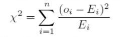
If X^2-statistic is large, then Object Oi is an outlier.
A low value for chi-square means there is a high correlation between your two sets of data. In theory, if your observed and expected values were equal (“no difference”) then chi-square would be zero — an event that is unlikely to happen in real life. You could take your calculated chi-square value and compare it to a critical value from a chi-square table. If the chi-square value is more than the critical value, then there is a significant difference.
A chi-square statistic is one way to show a relationship between two categorical variables. In statistics, there are two types of variables: numerical (countable) variables and non-numerical (categorical) variables. The chi-squared statistic is a single number that tells you how much difference exists between your observed counts and the counts you would expect if there were no relationship at all in the population.
[Omit] Parametric Methods III: Using mixture of parametric distributions
Outlier Detection is a big topic that can be expand for another article. Let me stop it here in Statistics topic.
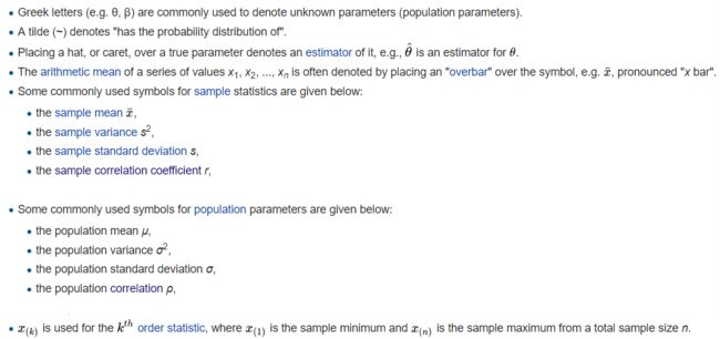
Statistics notation:
Note that statistics are quantities that we can calculate, and therefore do not depend on unknown parameters. Moveover, statistics have associated probability distributions, and we are sometimes interested in the distributions of statistics.
MLE: maximum likelihood estimate 最大似然估计
MSE: mean squared error 误差均方
RMSE: root mean squared error 误差均方根
r^2: coefficient of determination 确定系数
SE: standard error 标准误
SEM: standard error of the mean 均数的标准误
SS: sum of squares 平方和
SSE: sum of squared error of the prediction function
SSR: sum of squared residuals
SST: total sum of squares
