金融数值方法之回归计算-python实践
python的回归学习
前言
回归和插值是金融中常用的两种数学方法,本章将介绍关于回归的一些常用方法和代码。
一、回归是什么
回归是一种高效的求解函数近似值的工具,不仅对一维函数适用,同样也适用于高维函数。
最小化回归问题表达如下:

在回归的计算中,常用的范式为np.polyfit()、np.polyval()、np.linalg.lstsq()。
二、回归计算的具体实现
首先进行一些准备工作
import numpy as np
import matplotlib.pyplot as plt
from pylab import plt,mpl
plt.style.use('seaborn')
mpl.rcParams['font.family']='serif'
def f(x):
    return np.sin(x)+0.5*x
def create_plot(x,y,styles,labels,axlabels):
    plt.figure(figsize=(12,10))
    for i in range(len(x)):
        plt.plot(x[i],y[i],styles[i],label=labels[i])
        plt.xlabel(axlabels[0])
        plt.ylabel(axlabels[1])
    plt.legend(loc=0)
x=np.linspace(-2*np.pi,2*np.pi,50)
create_plot([x],[f(x)],['r'],['f(x)'],['x','f(x)'])
得到一个自定义的函数,如下所示:

1.单项式的回归
res=np.polyfit(x,f(x),deg=1,full=True)
print(res)
print('-'*108)
print(res[0])
得到参数
(array([ 4.28841952e-01, -5.29906205e-17]), array([21.03238686]), 2, array([1., 1.]), 1.1102230246251565e-14)
------------------------------------------------------------------------------------------------------------
[ 4.28841952e-01 -5.29906205e-17]
使用回归参数求值:
ry=np.polyval(res[0],x)
ry
array([-2.69449345, -2.58451412, -2.4745348 , -2.36455548, -2.25457615,
       -2.14459683, -2.0346175 , -1.92463818, -1.81465885, -1.70467953,
       -1.5947002 , -1.48472088, -1.37474156, -1.26476223, -1.15478291,
       -1.04480358, -0.93482426, -0.82484493, -0.71486561, -0.60488628,
       -0.49490696, -0.38492764, -0.27494831, -0.16496899, -0.05498966,
        0.05498966,  0.16496899,  0.27494831,  0.38492764,  0.49490696,
        0.60488628,  0.71486561,  0.82484493,  0.93482426,  1.04480358,
        1.15478291,  1.26476223,  1.37474156,  1.48472088,  1.5947002 ,
        1.70467953,  1.81465885,  1.92463818,  2.0346175 ,  2.14459683,
        2.25457615,  2.36455548,  2.4745348 ,  2.58451412,  2.69449345])
create_plot([x,x],[f(x),ry],['b','r.'],['f(x)','regression'],['x','f(x)'])
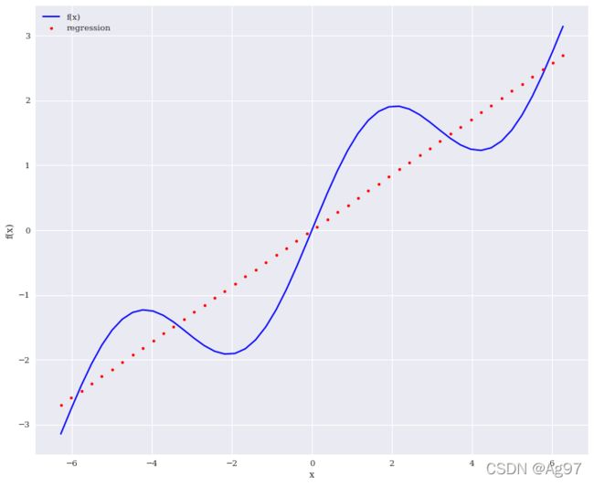
不太理想,使用五次单项式进行回归
res=np.polyfit(x,f(x),deg=5,full=True)
ry=np.polyval(res[0],x)
create_plot([x,x],[f(x),ry],['b','r.'],['f(x)','regression'],['x','f(x)'])

使用七次单项式进行回归:
res=np.polyfit(x,f(x),deg=7,full=True)
ry=np.polyval(res[0],x)
np.allclose(f(x),x)
False
false说明回归数值与原来的数值不是一样的。
计算mse
# mse计算
np.mean((f(x)-ry)**2)
0.00177691347595176
create_plot([x,x],[f(x),ry],['b','r.'],['f(x)','regression'],['x','f(x)'])

2.单独基函数
单独的基函数
np.linalg.lstsq
numpy.linalg.lstsq(a, b, rcond=‘warn’)
将least-squares解返回线性矩阵方程。
lstsq的输出包括四部分:回归系数、残差平方和、自变量X的秩、X的奇异值。一般只需要回归系数就可以了。
matrix=np.zeros((3+1,len(x)))
matrix[3,:]=x**3
matrix[2,:]=x**2
matrix[1,:]=x**1
matrix[0,:]=x**0
reg=np.linalg.lstsq(matrix.T,f(x),rcond=None)
reg[0].round(4)
ry=np.dot(reg[0].round(4),matrix)
ry
array([-2.19670554, -2.20978519, -2.2100222 , -2.19796307, -2.17415429,
       -2.13914236, -2.09347378, -2.03769503, -1.97235262, -1.89799303,
       -1.81516277, -1.72440833, -1.6262762 , -1.52131289, -1.41006488,
       -1.29307866, -1.17090075, -1.04407762, -0.91315578, -0.77868173,
       -0.64120195, -0.50126293, -0.35941119, -0.21619321, -0.07215549,
        0.07215549,  0.21619321,  0.35941119,  0.50126293,  0.64120195,
        0.77868173,  0.91315578,  1.04407762,  1.17090075,  1.29307866,
        1.41006488,  1.52131289,  1.6262762 ,  1.72440833,  1.81516277,
        1.89799303,  1.97235262,  2.03769503,  2.09347378,  2.13914236,
        2.17415429,  2.19796307,  2.2100222 ,  2.20978519,  2.19670554])
create_plot([x,x],[f(x),ry],['b','r.'],['f(x)','regression'],['x','f(x)'])

不太理想,将基函数中引入sinx函数
matrix[3,:]=np.sin(x)
reg=np.linalg.lstsq(matrix.T,f(x),rcond=None)
ry=np.dot(reg[0].round(4),matrix)
np.allclose(f(x),ry)
np.mean((f(x)-ry)**2)
create_plot([x,x],[f(x),ry],['b','r.'],['f(x)','regression'],['x','f(x)'])

3.有噪声的数据
# 有噪声的数据
xn=np.linspace(-2*np.pi,2*np.pi,50)
xn=xn+0.15*np.random.standard_normal(len(xn))
yn=f(xn)+0.15*np.random.standard_normal(len(xn))
reg=np.polyfit(xn,yn,7)
ry=np.polyval(reg,xn)
ry
array([-3.0627005 , -2.60200449, -2.38959333, -2.14942554, -2.01409671,
       -1.50484513, -1.226107  , -1.17844569, -1.16512748, -1.23329004,
       -1.26882923, -1.38858866, -1.47419669, -1.59087693, -1.83814445,
       -1.81224556, -1.8320825 , -1.84258301, -1.60920776, -1.61014972,
       -1.38753972, -1.01243076, -0.97922089, -0.47757572, -0.26812475,
        0.47485607,  0.37666023,  0.83580311,  1.39354247,  1.4589287 ,
        1.47395115,  1.73692656,  1.82542423,  1.86622981,  1.91271619,
        1.82514849,  1.62685373,  1.71879336,  1.54893674,  1.29743082,
        1.21692138,  1.21670403,  1.21887745,  1.34122101,  1.48378654,
        1.68455375,  2.39712865,  2.67237991,  3.06596453,  3.46057519])
create_plot([xn,xn],[yn,ry],['b','r.'],['f(xn)','regression'],['xn','f(xn)'])

4.未排序的数据
# 未排序的数据
xu=np.random.rand(50)*4*np.pi-2*np.pi
yu=f(xu)
reg=np.polyfit(xu,yu,5)
ry=np.polyval(reg,xu)
create_plot([xu,xu],[f(xu),ry],['b.','ro'],['f(xu)','regression'],['xu','f(xu)'])

5.多维的数据
# 多维
def fm(p):
    x,y=p
    return np.sin(x)+0.25*x+np.sqrt(y)+0.05*y**2
x=np.linspace(0,10,20)
y=np.linspace(0,10,20)
X,Y=np.meshgrid(x,y)
z=fm((X,Y))
x=X.flatten()
y=Y.flatten()
from mpl_toolkits.mplot3d import Axes3D
fig=plt.figure(figsize=(12,10))
ax=fig.gca(projection='3d')
surf=ax.plot_surface(X,Y,z,rstride=2,cstride=2,cmap='coolwarm',linewidth=0.5,
                    antialiased=True)
ax.set_xlabel('x')
ax.set_ylabel('y')
ax.set_zlabel('f(x,y)')

matrix=np.zeros((len(x),6+1))
matrix[:,6]=np.sqrt(y)
matrix[:,5]=np.sin(x)
matrix[:,4]=y**2
matrix[:,3]=x**2
matrix[:,2]=y
matrix[:,1]=x
matrix[:,0]=1
reg=np.linalg.lstsq(matrix,fm((x,y)),rcond=None)
rz=np.dot(matrix,reg[0].round(4)).reshape(20,20)
from mpl_toolkits.mplot3d import Axes3D
fig=plt.figure(figsize=(12,10))
ax=fig.gca(projection='3d')
surf1=ax.plot_surface(X,Y,z,rstride=2,cstride=2,cmap='coolwarm',linewidth=0.5,
                    antialiased=True)
surf2=ax.plot_wireframe(X,Y,rz,rstride=2,cstride=2,label='regression')
ax.set_xlabel('x')
ax.set_ylabel('y')
ax.set_zlabel('f(x,y)')
ax.legend()
fig.colorbar(surf,shrink=0.5,aspect=5)

总结
金融数值方法中的回归计算。