简述python在量化金融中应用_Python金融量化
Python股票数据分析
最近在学习基于python的股票数据分析,其中主要用到了tushare和seaborn。tushare是一款财经类数据接口包,国内的股票数据还是比较全的
官网地址:http://tushare.waditu.com/index.html#id5。seaborn则是一款绘图库,通过seaborn可以轻松地画出简洁漂亮的图表,而且库本身具有一定的统计功能。
导入的模块:
import matplotlib.pyplot as plt
import seaborn as sns
import seaborn.linearmodels as snsl
from datetime import datetime
import tushare as ts
代码部分:
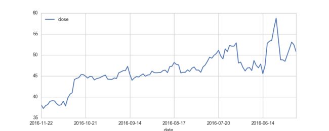
股票收盘价走势曲线
sns.set_style("whitegrid")
end = datetime.today() #开始时间结束时间,选取最近一年的数据
start = datetime(end.year-1,end.month,end.day)
end = str(end)[0:10]
start = str(start)[0:10]
stock = ts.get_hist_data('300104',start,end)#选取一支股票
stock['close'].plot(legend=True ,figsize=(10,4))
plt.show()
股票日线
同理,可以做出5日均线、10日均线以及20日均线
stock[['close','ma5','ma10','ma20']].plot(legend=True ,figsize=(10,4))
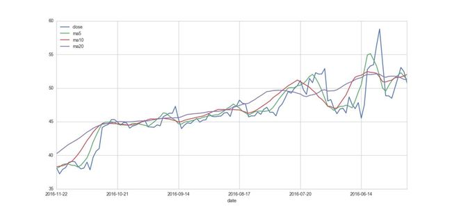
日线、5日均线、10日均线、20日均线
股票每日涨跌幅度
stock['Daily Return'] = stock['close'].pct_change()
stock['Daily Return'].plot(legend=True,figsize=(10,4))
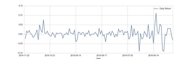
每日涨跌幅
核密度估计
sns.kdeplot(stock['Daily Return'].dropna())
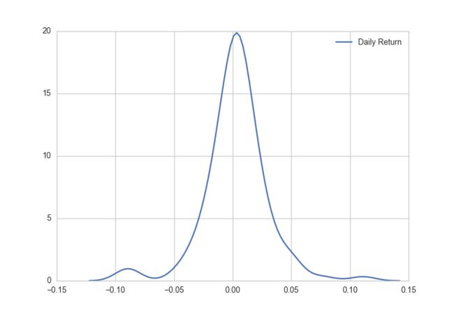
核密度估计
核密度估计+统计柱状图
sns.distplot(stock['Daily Return'].dropna(),bins=100)
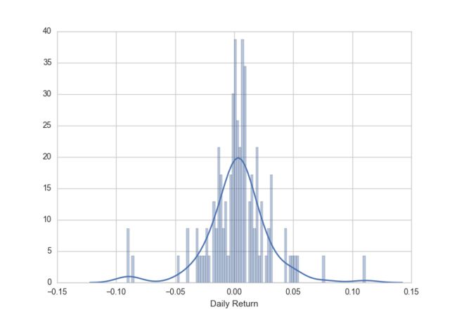
核密度+柱状图
两支股票的皮尔森相关系数
sns.jointplot(stock['Daily Return'],stock['Daily Return'],alpha=0.2)
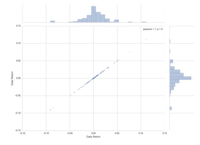
皮尔森相关系数
多只股票相关性计算
stock_lis=['300113','300343','300295','300315`] #随便选取了四支互联网相关的股票
df=pd.DataFrame()
for stock in stock_lis: closing_df = ts.get_hist_data(stock,start,end)['close'] df = df.join(pd.DataFrame({stock:closing_df}),how='outer')
tech_rets = df.pct_change()
snsl.corrplot(tech_rets.dropna())
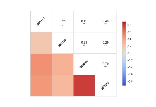
相关性
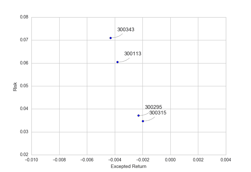
简单地计算股票的收益与风险,衡量股票收益与风险的数值分别为股票涨跌的平均值以及标准差,平均值为正则说明收益是正的,标准差越大则说明股票波动大,风险也大。
rets = tech_rets.dropna()
plt.scatter(rets.mean(),rets.std())
plt.xlabel('Excepted Return')
plt.ylabel('Risk')
for label,x,y in zip(rets.columns,rets.mean(),rets.std()):#添加标注 plt.annotate( label, xy =(x,y),xytext=(15,15), textcoords = 'offset points', arrowprops = dict(arrowstyle = '-',connectionstyle = 'arc3,rad=-0.3'))
声明:本文由入驻搜狐公众平台的作者撰写,除搜狐官方账号外,观点仅代表作者本人,不代表搜狐立场。
用Python分析公开数据选出高送转预期股票
根据以往的经验,每年年底都会有一波高送转预期行情。今天,米哥就带大家实践一下如何利用tushare实现高送转预期选股。
本文主要是讲述选股的思路方法,选股条件和参数大家可以根据米哥提供的代码自行修改。
1. 选股原理
一般来说,具备高送转预期的个股,都具有总市值低、每股公积金高、每股收益大,流通股本少的特点。当然,也还有其它的因素,比如当前股价、经营收益变动情况、以及以往分红送股习惯等等。
这里我们暂时只考虑每股公积金、每股收益、流通股本和总市值四个因素,将公积金大于等于5元,每股收益大于等于5毛,流通股本在3亿以下,总市值在100亿以内作为高送转预期目标(这些参数大家可根据自己的经验随意调整)。
2. 数据准备
首先要导入tushare:
import tushare as ts
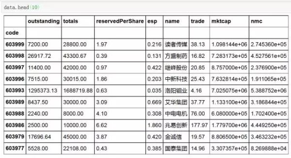
调取股票基本面数据和行情数据
# 基本面数据
basic = ts.get_stock_basics()
# 行情和市值数据
hq = ts.get_today_all()
3. 数据清洗整理
对获取到的数据进行清洗和整理,只保留需要的字段。(其它字段及含义,请参考 http:// tushare.org文档)
#当前股价,如果停牌则设置当前价格为上一个交易日股价
hq['trade'] = hq.apply(lambda x:x.settlement if x.trade==0 else x.trade, axis=1)
#分别选取流通股本,总股本,每股公积金,每股收益
basedata = basic[['outstanding', 'totals', 'reservedPerShare', 'esp']]
#选取股票代码,名称,当前价格,总市值,流通市值
hqdata = hq[['code', 'name', 'trade', 'mktcap', 'nmc']]
#设置行情数据code为index列
hqdata = hqdata.set_index('code')
#合并两个数据表
data = basedata.merge(hqdata, left_index=True, right_index=True)
4. 选股条件
根据上文提到的选股参数和条件,我们对数据进一步处理。
将总市值和流通市值换成亿元单位
data['mktcap'] = data['mktcap'] / 10000
data['nmc'] = data['nmc'] / 10000
设置参数和过滤值(此次各自调整)
#每股公积金>=5
res = data.reservedPerShare >= 5
#流通股本<=3亿
out = data.outstanding <= 30000
#每股收益>=5毛
eps = data.esp >= 0.5
#总市值<100亿
mktcap = data.mktcap <= 100
取并集结果:
allcrit = res & out & eps & mktcap
selected = data[allcrit]
具有高送转预期股票的结果呈现:
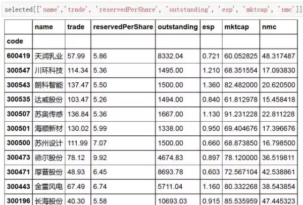
以上字段的含义分别为:股票名称、收盘价格、每股公积金、流通股本、每股收益(应该为eps,之前发布笔误)、总市值和流通市值。
https://zhuanlan.zhihu.com/p/23829205
Python 金叉判定


defjincha(context, bar_dict, his):#站上5日线
defzs5(context, bar_dict, his):
ma_n= pd.rolling_mean(his, 5)
temp= his -ma_n
#temp_s包含了前一天站上五日线得股票代码
temp_s= list(temp[temp>0].iloc[-1,:].dropna().index)returntemp_s#站上10日线
defzs10(context, bar_dict, his):
ma_n= pd.rolling_mean(his, 10)
temp= his -ma_n
temp_s= list(temp[temp>0].iloc[-1,:].dropna().index)returntemp_s#金叉突破
defjc(context, bar_dict, his):
mas= pd.rolling_mean(his,5)
mal= pd.rolling_mean(his, 10)
temp= mas -mal#temp_jc昨天大于0股票代码
#temp_r前天大于0股票代码
temp_jc= list(temp[temp>0].iloc[-1,:].dropna().index)
temp_r= list(temp[temp>0].iloc[-2,:].dropna().index)
temp=[]for stock intemp_jc:if stock not intemp_r:
temp.append(stock)returntemp#求三种条件下的股票代码交集
con1=zs5(context, bar_dict, his)
con2=zs10(context, bar_dict, his)
con3=jc(context, bar_dict, his)
tar_list=[con1,con2,con3]
tarstock=tar_list[0]for i intar_list:
tarstock=list(set(tarstock).intersection(set(i)))return tarstock
View Code
Python 过滤次新股、停牌、涨跌停
#过滤次新股、是否涨跌停、是否停牌等条件
deffilcon(context,bar_dict,tar_list):defzdt_trade(stock, context, bar_dict):
yesterday= history(2,'1d', 'close')[stock].values[-1]
zt= round(1.10 * yesterday,2)
dt= round(0.99 * yesterday,2)#last最后交易价
return dt < bar_dict[stock].last
filstock=[]for stock intar_list:
con1= ipo_days(stock,context.now) > 60con2=bar_dict[stock].is_trading
con3=zdt_trade(stock,context,bar_dict)if con1 & con2 &con3:
filstock.append(stock)return filstock
View Code
Python 按平均持仓市值调仓
#按平均持仓市值调仓
deffor_balance(context, bar_dict):#mvalues = context.portfolio.market_value
#avalues = context.portfolio.portfolio_value
#per = mvalues / avalues
hlist =[]for stock incontext.portfolio.positions:#获取股票及对应持仓市值
hlist.append([stock,bar_dict[stock].last *context.portfolio.positions[stock].quantity])ifhlist:#按持仓市值由大到小排序
hlist = sorted(hlist,key=lambda x:x[1], reverse=True)
temp=0for li inhlist:#计算持仓总市值
temp += li[1]for li inhlist:#平均各股持仓市值
ifbar_dict[li[0]].is_trading:
order_target_value(li[0], temp/len(hlist))return
View Code
Python PCA主成分分析算法
Python主成分分析算法的作用是提取样本的主要特征向量,从而实现数据降维的目的。
#-*- coding: utf-8 -*-
"""Created on Sun Feb 28 10:04:26 2016
PCA source code
@author: liudiwei"""
importnumpy as npimportpandas as pdimportmatplotlib.pyplot as plt#计算均值,要求输入数据为numpy的矩阵格式,行表示样本数,列表示特征
defmeanX(dataX):return np.mean(dataX,axis=0)#axis=0表示按照列来求均值,如果输入list,则axis=1
#计算方差,传入的是一个numpy的矩阵格式,行表示样本数,列表示特征
defvariance(X):
m, n=np.shape(X)
mu=meanX(X)
muAll= np.tile(mu, (m, 1))
X1= X -muAll
variance= 1./m * np.diag(X1.T *X1)returnvariance#标准化,传入的是一个numpy的矩阵格式,行表示样本数,列表示特征
defnormalize(X):
m, n=np.shape(X)
mu=meanX(X)
muAll= np.tile(mu, (m, 1))
X1= X -muAll
X2= np.tile(np.diag(X.T * X), (m, 1))
XNorm= X1/X2returnXNorm"""参数:
- XMat:传入的是一个numpy的矩阵格式,行表示样本数,列表示特征
- k:表示取前k个特征值对应的特征向量
返回值:
- finalData:参数一指的是返回的低维矩阵,对应于输入参数二
- reconData:参数二对应的是移动坐标轴后的矩阵"""
defpca(XMat, k):
average=meanX(XMat)
m, n=np.shape(XMat)
data_adjust=[]
avgs= np.tile(average, (m, 1))
data_adjust= XMat -avgs
covX= np.cov(data_adjust.T) #计算协方差矩阵
featValue, featVec= np.linalg.eig(covX) #求解协方差矩阵的特征值和特征向量
index = np.argsort(-featValue) #按照featValue进行从大到小排序
finalData =[]if k >n:print "k must lower than feature number"
return
else:#注意特征向量时列向量,而numpy的二维矩阵(数组)a[m][n]中,a[1]表示第1行值
selectVec = np.matrix(featVec.T[index[:k]]) #所以这里需要进行转置
finalData = data_adjust *selectVec.T
reconData= (finalData * selectVec) +averagereturnfinalData, reconDatadefloaddata(datafile):return np.array(pd.read_csv(datafile,sep="\t",header=-1)).astype(np.float)defplotBestFit(data1, data2):
dataArr1=np.array(data1)
dataArr2=np.array(data2)
m=np.shape(dataArr1)[0]
axis_x1=[]
axis_y1=[]
axis_x2=[]
axis_y2=[]for i inrange(m):
axis_x1.append(dataArr1[i,0])
axis_y1.append(dataArr1[i,1])
axis_x2.append(dataArr2[i,0])
axis_y2.append(dataArr2[i,1])
fig=plt.figure()
ax= fig.add_subplot(111)
ax.scatter(axis_x1, axis_y1, s=50, c='red', marker='s')
ax.scatter(axis_x2, axis_y2, s=50, c='blue')
plt.xlabel('x1'); plt.ylabel('x2');
plt.savefig("outfile.png")
plt.show()#简单测试#数据来源:http://www.cnblogs.com/jerrylead/archive/2011/04/18/2020209.html
deftest():
X= [[2.5, 0.5, 2.2, 1.9, 3.1, 2.3, 2, 1, 1.5, 1.1],
[2.4, 0.7, 2.9, 2.2, 3.0, 2.7, 1.6, 1.1, 1.6, 0.9]]
XMat=np.matrix(X).T
k= 2
returnpca(XMat, k)#根据数据集data.txt
defmain():
datafile= "data.txt"XMat=loaddata(datafile)
k= 2
returnpca(XMat, k)if __name__ == "__main__":
finalData, reconMat=main()
plotBestFit(finalData, reconMat)
View Code
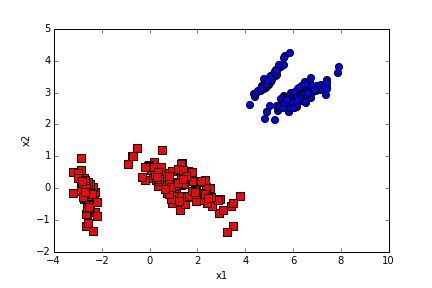
经过主成分降维的数据如红色图案所示,蓝色的是恢复的原始数据。可以看到经过降维的数据样本差异更加明显。
Python KNN最近邻分类算法
KNN最近邻算法:利用向量之间的距离来分类。
步骤:
第一步:计算新样本与已知分类样本之间的距离。
第二步:将所求距离按从小到大排列。
第三步:选取距离最近的k个样本。
第四步:将新样本归为以上k个样本大多数中的一类。
以下为KNN最近邻分类算法的python代码:
第一部分:KNN分类代码
#-*- coding: utf-8 -*-
"""Created on Mon Feb 22 13:21:22 2016
K-NearestNeighbor"""
importnumpy as npimportoperatorclassKNNClassifier():"""This is a Nearest Neighbor classifier."""
#定义k的值
def __init__(self, k=3):
self._k=k#计算新样本与已知分类样本的距离并从小到大排列
def_calEDistance(self, inSample, dataset):
m=dataset.shape[0]
diffMat= np.tile(inSample, (m,1)) -dataset
sqDiffMat= diffMat**2 #每个元素平方
sqDistances = sqDiffMat.sum(axis = 1) #求和
distances = sqDistances ** 0.5 #开根号
return distances.argsort() #按距离的从小到达排列的下标值
def_classify0(self, inX, dataSet, labels):
k=self._k
dataSetSize=dataSet.shape[0]
diffMat= np.tile(inX, (dataSetSize,1)) -dataSet
sqDiffMat= diffMat**2sqDistances= sqDiffMat.sum(axis=1)
distances= sqDistances**0.5sortedDistIndicies=distances.argsort()
classCount={}for i inrange(k):
voteIlabel=labels[sortedDistIndicies[i]]
classCount[voteIlabel]= classCount.get(voteIlabel,0) + 1sortedClassCount= sorted(classCount.iteritems(), key=operator.itemgetter(1), reverse=True)returnsortedClassCount[0][0]#对一个样本进行分类
def_classify(self, sample, train_X, train_y):#数据类型检测
if isinstance(sample, np.ndarray) andisinstance(train_X, np.ndarray) \andisinstance(train_y, np.ndarray):pass
else:try:
sample=np.array(sample)
train_X=np.array(train_X)
train_y=np.array(train_y)except:raise TypeError("numpy.ndarray required for train_X and ..")
sortedDistances=self._calEDistance(sample, train_X)
classCount={}for i inrange(self._k):
oneVote= train_y[sortedDistances[i]] #获取最近的第i个点的类别
classCount[oneVote] = classCount.get(oneVote, 0) + 1sortedClassCount=sorted(classCount.iteritems(),\
key=operator.itemgetter(1), reverse=True)#print "the sample :", sample, "is classified as",sortedClassCount[0][0]
returnsortedClassCount[0][0]defclassify(self, test_X, train_X, train_y):
results=[]#数据类型检测
if isinstance(test_X, np.ndarray) andisinstance(train_X, np.ndarray) \andisinstance(train_y, np.ndarray):pass
else:try:
test_X=np.array(test_X)
train_X=np.array(train_X)
train_y=np.array(train_y)except:raise TypeError("numpy.ndarray required for train_X and ..")
d=len(np.shape(test_X))if d == 1:
sample=test_X
result=self._classify(sample, train_X, train_y)
results.append(result)else:for i inrange(len(test_X)):
sample=test_X[i]
result=self._classify(sample, train_X, train_y)
results.append(result)returnresultsif __name__=="__main__":
train_X= [[1, 2, 0, 1, 0],
[0,1, 1, 0, 1],
[1, 0, 0, 0, 1],
[2, 1, 1, 0, 1],
[1, 1, 0, 1, 1]]
train_y= [1, 1, 0, 0, 0]
clf= KNNClassifier(k = 3)
sample= [[1,2,0,1,0],[1,2,0,1,1]]
result= clf.classify(sample, train_X, train_y)
View Code
第二部分:KNN测试代码
#-*- coding: utf-8 -*-
"""Created on Mon Feb 22 13:21:22 2016
K-NearestNeighbor"""
importnumpy as npimportoperatorclassKNNClassifier():"""This is a Nearest Neighbor classifier."""
#定义k的值
def __init__(self, k=3):
self._k=k#计算新样本与已知分类样本的距离并从小到大排列
def_calEDistance(self, inSample, dataset):
m=dataset.shape[0]
diffMat= np.tile(inSample, (m,1)) -dataset
sqDiffMat= diffMat**2 #每个元素平方
sqDistances = sqDiffMat.sum(axis = 1) #求和
distances = sqDistances ** 0.5 #开根号
return distances.argsort() #按距离的从小到达排列的下标值
def_classify0(self, inX, dataSet, labels):
k=self._k
dataSetSize=dataSet.shape[0]
diffMat= np.tile(inX, (dataSetSize,1)) -dataSet
sqDiffMat= diffMat**2sqDistances= sqDiffMat.sum(axis=1)
distances= sqDistances**0.5sortedDistIndicies=distances.argsort()
classCount={}for i inrange(k):
voteIlabel=labels[sortedDistIndicies[i]]
classCount[voteIlabel]= classCount.get(voteIlabel,0) + 1sortedClassCount= sorted(classCount.iteritems(), key=operator.itemgetter(1), reverse=True)returnsortedClassCount[0][0]#对一个样本进行分类
def_classify(self, sample, train_X, train_y):#数据类型检测
if isinstance(sample, np.ndarray) andisinstance(train_X, np.ndarray) \andisinstance(train_y, np.ndarray):pass
else:try:
sample=np.array(sample)
train_X=np.array(train_X)
train_y=np.array(train_y)except:raise TypeError("numpy.ndarray required for train_X and ..")
sortedDistances=self._calEDistance(sample, train_X)
classCount={}for i inrange(self._k):
oneVote= train_y[sortedDistances[i]] #获取最近的第i个点的类别
classCount[oneVote] = classCount.get(oneVote, 0) + 1sortedClassCount=sorted(classCount.iteritems(),\
key=operator.itemgetter(1), reverse=True)#print "the sample :", sample, "is classified as",sortedClassCount[0][0]
returnsortedClassCount[0][0]defclassify(self, test_X, train_X, train_y):
results=[]#数据类型检测
if isinstance(test_X, np.ndarray) andisinstance(train_X, np.ndarray) \andisinstance(train_y, np.ndarray):pass
else:try:
test_X=np.array(test_X)
train_X=np.array(train_X)
train_y=np.array(train_y)except:raise TypeError("numpy.ndarray required for train_X and ..")
d=len(np.shape(test_X))if d == 1:
sample=test_X
result=self._classify(sample, train_X, train_y)
results.append(result)else:for i inrange(len(test_X)):
sample=test_X[i]
result=self._classify(sample, train_X, train_y)
results.append(result)returnresultsif __name__=="__main__":
train_X= [[1, 2, 0, 1, 0],
[0,1, 1, 0, 1],
[1, 0, 0, 0, 1],
[2, 1, 1, 0, 1],
[1, 1, 0, 1, 1]]
train_y= [1, 1, 0, 0, 0]
clf= KNNClassifier(k = 3)
sample= [[1,2,0,1,0],[1,2,0,1,1]]
result= clf.classify(sample, train_X, train_y)
View Code
Python 决策树算法(ID3 &C4.5)
决策树(Decision Tree)算法:按照样本的属性逐步进行分类,为了能够使分类更快、更有效。每一个新分类属性的选择依据可以是信息增益IG和信息增益率IGR,前者为最基本的ID3算法,后者为改进后的C4.5算法。
以ID3为例,其训练过程的编程思路如下:
(1)输入x、y(x为样本,y为label),行为样本,列为样本特征。
(2)计算信息增益IG,获取使IG最大的特征。
(3)获得删除最佳分类特征后的样本阵列。
(4)按照最佳分类特征的属性值将更新后的样本进行归类。
属性值1(x1,y1) 属性值2(x2,y2) 属性值(x3,y3)
(5)分别对以上类别重复以上操作直至到达叶节点(递归调用)。
叶节点的特征:
(1)所有的标签值y都一样。
(2)没有特征可以继续划分。
测试过程的编程思路如下:
(1)读取训练好的决策树。
(2)从根节点开始递归遍历整个决策树直到到达叶节点为止。
以下为具体代码,训练后的决策树结构为递归套用的字典,其是由特征值组成的索引加上label组成的。
#-*- coding: utf-8 -*-
"""Created on Mon Nov 07 09:06:37 2016
@author: yehx"""
#-*- coding: utf-8 -*-
"""Created on Sun Feb 21 12:17:10 2016
Decision Tree Source Code
@author: liudiwei"""
importosimportnumpy as npclassDecitionTree():"""This is a decision tree classifier."""
def __init__(self, criteria='ID3'):
self._tree=Noneif criteria == 'ID3' or criteria == 'C4.5':
self._criteria=criteriaelse:raise Exception("criterion should be ID3 or C4.5")def_calEntropy(slef, y):'''功能:_calEntropy用于计算香农熵 e=-sum(pi*log pi)
参数:其中y为数组array
输出:信息熵entropy'''n=y.shape[0]
labelCounts={}for label iny:if label not inlabelCounts.keys():
labelCounts[label]= 1
else:
labelCounts[label]+= 1entropy= 0.0
for key inlabelCounts:
prob= float(labelCounts[key])/n
entropy-= prob *np.log2(prob)returnentropydef_splitData(self, X, y, axis, cutoff):"""参数:X为特征,y为label,axis为某个特征的下标,cutoff是下标为axis特征取值值
输出:返回数据集中特征下标为axis,特征值等于cutoff的子数据集
先将特征列从样本矩阵里除去,然后将属性值为cutoff的数据归为一类"""ret=[]
featVec=X[:,axis]
n= X.shape[1] #特征个数
#除去第axis列特征后的样本矩阵
X = X[:,[i for i in range(n) if i!=axis]]for i inrange(len(featVec)):if featVec[i] ==cutoff:
ret.append(i)returnX[ret, :], y[ret]def_chooseBestSplit(self, X, y):"""ID3 & C4.5
参数:X为特征,y为label
功能:根据信息增益或者信息增益率来获取最好的划分特征
输出:返回最好划分特征的下标"""numFeat= X.shape[1]
baseEntropy=self._calEntropy(y)
bestSplit= 0.0best_idx= -1
for i inrange(numFeat):
featlist= X[:,i] #得到第i个特征对应的特征列
uniqueVals =set(featlist)
curEntropy= 0.0splitInfo= 0.0
for value inuniqueVals:
sub_x, sub_y=self._splitData(X, y, i, value)
prob= len(sub_y)/float(len(y)) #计算某个特征的某个值的概率
curEntropy += prob * self._calEntropy(sub_y) #迭代计算条件熵
splitInfo -= prob * np.log2(prob) #分裂信息,用于计算信息增益率
IG = baseEntropy -curEntropyif self._criteria=="ID3":if IG >bestSplit:
bestSplit=IG
best_idx=iif self._criteria=="C4.5":if splitInfo == 0.0:passIGR= IG/splitInfoif IGR >bestSplit:
bestSplit=IGR
best_idx=ireturnbest_idxdef_majorityCnt(self, labellist):"""参数:labellist是类标签,序列类型为list
输出:返回labellist中出现次数最多的label"""labelCount={}for vote inlabellist:if vote not inlabelCount.keys():
labelCount[vote]=0
labelCount[vote]+= 1sortedClassCount= sorted(labelCount.iteritems(), key=lambda x:x[1], \
reverse=True)returnsortedClassCount[0][0]def_createTree(self, X, y, featureIndex):"""参数:X为特征,y为label,featureIndex类型是元组,记录X特征在原始数据中的下标
输出:根据当前的featureIndex创建一颗完整的树"""labelList=list(y)#如果所有的标签都一样(叶节点),直接返回标签
if labelList.count(labelList[0]) ==len(labelList):returnlabelList[0]#如果没有特征可以继续划分,那么将所有的label归为大多数的一类,并返回标签
if len(featureIndex) ==0:returnself._majorityCnt(labelList)#返回最佳分类特征的下标
bestFeatIndex =self._chooseBestSplit(X,y)#返回最佳分类特征的索引
bestFeatAxis =featureIndex[bestFeatIndex]
featureIndex=list(featureIndex)#获得删除最佳分类特征索引后的列表
featureIndex.remove(bestFeatAxis)
featureIndex=tuple(featureIndex)
myTree={bestFeatAxis:{}}
featValues=X[:, bestFeatIndex]
uniqueVals=set(featValues)for value inuniqueVals:#对每个value递归地创建树
sub_X, sub_y =self._splitData(X,y, bestFeatIndex, value)
myTree[bestFeatAxis][value]=self._createTree(sub_X, sub_y, \
featureIndex)returnmyTreedeffit(self, X, y):"""参数:X是特征,y是类标签
注意事项:对数据X和y进行类型检测,保证其为array
输出:self本身"""
if isinstance(X, np.ndarray) andisinstance(y, np.ndarray):pass
else:try:
X=np.array(X)
y=np.array(y)except:raise TypeError("numpy.ndarray required for X,y")
featureIndex= tuple(['x'+str(i) for i in range(X.shape[1])])
self._tree=self._createTree(X,y,featureIndex)return self #allow using: clf.fit().predict()
def_classify(self, tree, sample):"""用训练好的模型对输入数据进行分类
注意:决策树的构建是一个递归的过程,用决策树分类也是一个递归的过程
_classify()一次只能对一个样本(sample)分类"""featIndex= tree.keys()[0] #得到数的根节点值
secondDict = tree[featIndex] #得到以featIndex为划分特征的结果
axis=featIndex[1:] #得到根节点特征在原始数据中的下标
key = sample[int(axis)] #获取待分类样本中下标为axis的值
valueOfKey = secondDict[key] #获取secondDict中keys为key的value值
if type(valueOfKey).__name__=='dict': #如果value为dict,则继续递归分类
returnself._classify(valueOfKey, sample)else:returnvalueOfKeydefpredict(self, X):if self._tree==None:raise NotImplementedError("Estimator not fitted, call `fit` first")#对X的类型进行检测,判断其是否是数组
ifisinstance(X, np.ndarray):pass
else:try:
X=np.array(X)except:raise TypeError("numpy.ndarray required for X")if len(X.shape) == 1:returnself._classify(self._tree, X)else:
result=[]for i inrange(X.shape[0]):
value=self._classify(self._tree, X[i])print str(i+1)+"-th sample is classfied as:", value
result.append(value)returnnp.array(result)defshow(self, outpdf):if self._tree==None:pass
#plot the tree using matplotlib
importtreePlotter
treePlotter.createPlot(self._tree, outpdf)if __name__=="__main__":
trainfile=r"data\train.txt"testfile=r"data\test.txt"
importsys
sys.path.append(r"F:\CSU\Github\MachineLearning\lib")importdataload as dload
train_x, train_y=dload.loadData(trainfile)
test_x, test_y=dload.loadData(testfile)
clf= DecitionTree(criteria="C4.5")
clf.fit(train_x, train_y)
result=clf.predict(test_x)
outpdf= r"tree.pdf"clf.show(outpdf)
View Code
Python K均值聚类
Python K均值聚类是一种无监督的机器学习算法,能够实现自动归类的功能。
算法步骤如下:
(1)随机产生K个分类中心,一般称为质心。
(2)将所有样本划分到距离最近的质心代表的分类中。(距离可以是欧氏距离、曼哈顿距离、夹角余弦等)
(3)计算分类后的质心,可以用同一类中所有样本的平均属性来代表新的质心。
(4)重复(2)(3)两步,直到满足以下其中一个条件:
1)分类结果没有发生改变。
2)最小误差(如平方误差)达到所要求的范围。
3)迭代总数达到设置的最大值。
常见的K均值聚类算法还有2分K均值聚类算法,其步骤如下:
(1)将所有样本作为一类。
(2)按照传统K均值聚类的方法将样本分为两类。
(3)对以上两类分别再分为两类,且分别计算两种情况下误差,仅保留误差更小的分类;即第(2)步产生的两类其中一类保留,另一类进行再次分类。
(4)重复对已有类别分别进行二分类,同理保留误差最小的分类,直到达到所需要的分类数目。
具体Python代码如下:
#-*- coding: utf-8 -*-
"""Created on Tue Nov 08 14:01:44 2016
K - means cluster"""
importnumpy as npclassKMeansClassifier():"this is a k-means classifier"
def __init__(self, k=3, initCent='random', max_iter=500):
self._k=k
self._initCent=initCent
self._max_iter=max_iter
self._clusterAssment=None
self._labels=None
self._sse=Nonedef_calEDist(self, arrA, arrB):"""功能:欧拉距离距离计算
输入:两个一维数组"""
return np.math.sqrt(sum(np.power(arrA-arrB, 2)))def_calMDist(self, arrA, arrB):"""功能:曼哈顿距离距离计算
输入:两个一维数组"""
return sum(np.abs(arrA-arrB))def_randCent(self, data_X, k):"""功能:随机选取k个质心
输出:centroids #返回一个m*n的质心矩阵"""n= data_X.shape[1] #获取特征的维数
centroids = np.empty((k,n)) #使用numpy生成一个k*n的矩阵,用于存储质心
for j inrange(n):
minJ=min(data_X[:, j])
rangeJ= float(max(data_X[:, j] -minJ))#使用flatten拉平嵌套列表(nested list)
centroids[:, j] = (minJ + rangeJ * np.random.rand(k, 1)).flatten()returncentroidsdeffit(self, data_X):"""输入:一个m*n维的矩阵"""
if not isinstance(data_X, np.ndarray) or\
isinstance(data_X, np.matrixlib.defmatrix.matrix):try:
data_X=np.asarray(data_X)except:raise TypeError("numpy.ndarray resuired for data_X")
m= data_X.shape[0] #获取样本的个数
#一个m*2的二维矩阵,矩阵第一列存储样本点所属的族的索引值,
#第二列存储该点与所属族的质心的平方误差
self._clusterAssment = np.zeros((m,2))if self._initCent == 'random':
self._centroids=self._randCent(data_X, self._k)
clusterChanged=Truefor _ in range(self._max_iter): #使用"_"主要是因为后面没有用到这个值
clusterChanged =Falsefor i in range(m): #将每个样本点分配到离它最近的质心所属的族
minDist = np.inf #首先将minDist置为一个无穷大的数
minIndex = -1 #将最近质心的下标置为-1
for j in range(self._k): #次迭代用于寻找最近的质心
arrA =self._centroids[j,:]
arrB=data_X[i,:]
distJI= self._calEDist(arrA, arrB) #计算误差值
if distJI minDist=distJI minIndex=jif self._clusterAssment[i,0] !=minIndex: clusterChanged=True self._clusterAssment[i,:]= minIndex, minDist**2 if not clusterChanged:#若所有样本点所属的族都不改变,则已收敛,结束迭代 break for i in range(self._k):#更新质心,将每个族中的点的均值作为质心 index_all = self._clusterAssment[:,0] #取出样本所属簇的索引值 value = np.nonzero(index_all==i) #取出所有属于第i个簇的索引值 ptsInClust = data_X[value[0]] #取出属于第i个簇的所有样本点 self._centroids[i,:] = np.mean(ptsInClust, axis=0) #计算均值 self._labels=self._clusterAssment[:,0] self._sse= sum(self._clusterAssment[:,1])def predict(self, X):#根据聚类结果,预测新输入数据所属的族 #类型检查 if notisinstance(X,np.ndarray):try: X=np.asarray(X)except:raise TypeError("numpy.ndarray required for X") m= X.shape[0]#m代表样本数量 preds =np.empty((m,))for i in range(m):#将每个样本点分配到离它最近的质心所属的族 minDist =np.inffor j inrange(self._k): distJI=self._calEDist(self._centroids[j,:], X[i,:])if distJI minDist=distJI preds[i]=jreturnpredsclassbiKMeansClassifier():"this is a binary k-means classifier" def __init__(self, k=3): self._k=k self._centroids=None self._clusterAssment=None self._labels=None self._sse=Nonedef_calEDist(self, arrA, arrB):"""功能:欧拉距离距离计算 输入:两个一维数组""" return np.math.sqrt(sum(np.power(arrA-arrB, 2)))deffit(self, X): m=X.shape[0] self._clusterAssment= np.zeros((m,2)) centroid0= np.mean(X, axis=0).tolist() centList=[centroid0]for j in range(m):#计算每个样本点与质心之间初始的平方误差 self._clusterAssment[j,1] =self._calEDist(np.asarray(centroid0), \ X[j,:])**2 while (len(centList) lowestSSE=np.inf#尝试划分每一族,选取使得误差最小的那个族进行划分 for i inrange(len(centList)): index_all= self._clusterAssment[:,0] #取出样本所属簇的索引值 value = np.nonzero(index_all==i) #取出所有属于第i个簇的索引值 ptsInCurrCluster = X[value[0],:] #取出属于第i个簇的所有样本点 clf = KMeansClassifier(k=2) clf.fit(ptsInCurrCluster)#划分该族后,所得到的质心、分配结果及误差矩阵 centroidMat, splitClustAss =clf._centroids, clf._clusterAssment sseSplit= sum(splitClustAss[:,1]) index_all=self._clusterAssment[:,0] value= np.nonzero(index_all==i) sseNotSplit= sum(self._clusterAssment[value[0],1])if (sseSplit + sseNotSplit) bestCentToSplit=i bestNewCents=centroidMat bestClustAss=splitClustAss.copy() lowestSSE= sseSplit +sseNotSplit#该族被划分成两个子族后,其中一个子族的索引变为原族的索引 #另一个子族的索引变为len(centList),然后存入centList bestClustAss[np.nonzero(bestClustAss[:,0]==1)[0],0]=len(centList) bestClustAss[np.nonzero(bestClustAss[:,0]==0)[0],0]=bestCentToSplit centList[bestCentToSplit]=bestNewCents[0,:].tolist() centList.append(bestNewCents[1,:].tolist()) self._clusterAssment[np.nonzero(self._clusterAssment[:,0]==\ bestCentToSplit)[0],:]=bestClustAss self._labels=self._clusterAssment[:,0] self._sse= sum(self._clusterAssment[:,1]) self._centroids=np.asarray(centList)def predict(self, X):#根据聚类结果,预测新输入数据所属的族 #类型检查 if notisinstance(X,np.ndarray):try: X=np.asarray(X)except:raise TypeError("numpy.ndarray required for X") m= X.shape[0]#m代表样本数量 preds =np.empty((m,))for i in range(m):#将每个样本点分配到离它最近的质心所属的族 minDist =np.inffor j inrange(self._k): distJI=self._calEDist(self._centroids[j,:],X[i,:])if distJI minDist=distJI preds[i]=jreturn preds View Code Python股票历史涨跌幅数据获取 股票涨跌幅数据是量化投资学习的基本数据资料之一,下面以Python代码编程为工具,获得所需要的历史数据。主要步骤有: (1) #按照市值从小到大的顺序活得N支股票的代码; (2) #分别对这一百只股票进行100支股票操作; (3) #获取从2016.05.01到2016.11.17的涨跌幅数据; (4) #选取记录大于40个的数据,去除次新股; (5) #将文件名名为“股票代码.csv”。 具体代码如下: #-*- coding: utf-8 -*- """Created on Thu Nov 17 23:04:33 2016 获取股票的历史涨跌幅,并分别存为csv格式 @author: yehx""" importnumpy as npimportpandas as pd#按照市值从小到大的顺序活得100支股票的代码 df =get_fundamentals( query(fundamentals.eod_derivative_indicator.market_cap) .order_by(fundamentals.eod_derivative_indicator.market_cap.asc()) .limit(100),'2016-11-17', '1y')#分别对这一百只股票进行100支股票操作#获取从2016.05.01到2016.11.17的涨跌幅数据#选取记录大于40个的数据,去除次新股#将文件名名为“股票代码.csv” for stock in range(100): priceChangeRate= get_price_change_rate(df['market_cap'].columns[stock], '20160501', '20161117')if priceChangeRate isNone: openDays=0else: openDays=len(priceChangeRate)if openDays > 40: tempPrice= priceChangeRate[39:(openDays - 1)]for rate inrange(len(tempPrice)): tempPrice[rate]= "%.3f" %tempPrice[rate] fileName= ''fileName= fileName.join(df['market_cap'].columns[i].split('.')) + '.csv'fileName tempPrice.to_csv(fileName) View Code Python Logistic 回归分类 Logistic回归可以认为是线性回归的延伸,其作用是对二分类样本进行训练,从而对达到预测新样本分类的目的。 假设有一组已知分类的MxN维样本X,M为样本数,N为特征维度,其相应的已知分类标签为Mx1维矩阵Y。那么Logistic回归的实现思路如下: (1)用一组权重值W(Nx1)对X的特征进行线性变换,得到变换后的样本X’(Mx1),其目标是使属于不同分类的样本X’存在一个明显的一维边界。 (2)然后再对样本X’进一步做函数变换,从而使处于一维边界两测的值变换到相应的范围之内。 (3)训练过程就是通过改变W尽可能使得到的值位于一维边界两侧,并且与已知分类相符。 (4)对于Logistic回归,就是将原样本的边界变换到x=0这个边界。 下面是Logistic回归的典型代码: #-*- coding: utf-8 -*- """Created on Wed Nov 09 15:21:48 2016 Logistic回归分类""" importnumpy as npclassLogisticRegressionClassifier():def __init__(self): self._alpha=None#定义一个sigmoid函数 def_sigmoid(self, fx):return 1.0/(1 + np.exp(-fx))#alpha为步长(学习率);maxCycles最大迭代次数 def_gradDescent(self, featData, labelData, alpha, maxCycles): dataMat= np.mat(featData) #size: m*n labelMat = np.mat(labelData).transpose() #size: m*1 m, n =np.shape(dataMat) weigh= np.ones((n, 1))for i inrange(maxCycles): hx= self._sigmoid(dataMat *weigh) error= labelMat - hx #size:m*1 weigh = weigh + alpha * dataMat.transpose() * error#根据误差修改回归系数 returnweigh#使用梯度下降方法训练模型,如果使用其它的寻参方法,此处可以做相应修改 def fit(self, train_x, train_y, alpha=0.01, maxCycles=100):returnself._gradDescent(train_x, train_y, alpha, maxCycles)#使用学习得到的参数进行分类 defpredict(self, test_X, test_y, weigh): dataMat=np.mat(test_X) labelMat= np.mat(test_y).transpose() #使用transpose()转置 hx = self._sigmoid(dataMat*weigh) #size:m*1 m =len(hx) error= 0.0 for i inrange(m):if int(hx[i]) > 0.5:print str(i+1)+'-th sample', int(labelMat[i]), 'is classfied as: 1' if int(labelMat[i]) != 1: error+= 1.0 print "classify error." else:print str(i+1)+'-th sample', int(labelMat[i]), 'is classfied as: 0' if int(labelMat[i]) !=0: error+= 1.0 print "classify error."error_rate= error/mprint "error rate is:", "%.4f" %error_ratereturn error_rate View Code Python 朴素贝叶斯(Naive Bayes)分类 Naïve Bayes 分类的核心是计算条件概率P(y|x),其中y为类别,x为特征向量。其意义是在x样本出现时,它被划分为y类的可能性(概率)。通过计算不同分类下的概率,进而把样本划分到概率最大的一类。 根据条件概率的计算公式可以得到: P(y|x) = P(y)*P(x|y)/P(x)。 由于在计算不同分类概率是等式右边的分母是相同的,所以只需比较分子的大小。并且,如果各个样本特征是独立分布的,那么p(x |y)等于p(xi|y)相乘。 下面以文本分类来介绍Naïve Bayes分类的应用。其思路如下: (1)建立词库,即无重复的单词表。 (2)分别计算词库中类别标签出现的概率P(y)。 (3)分别计算各个类别标签下不同单词出现的概率P(xi|y)。 (4)在不同类别下,将待分类样本各个特征出现概率((xi|y)相乘,然后在乘以对应的P(y)。 (5)比较不同类别下(4)中结果,将待分类样本分到取值最大的类别。 下面是Naïve Bayes 文本分类的Python代码,其中为了方便计算,程序中借助log对数函数将乘法转化为了加法。 #-*- coding: utf-8 -*- """Created on Mon Nov 14 11:15:47 2016 Naive Bayes Clssification""" #-*- coding: utf-8 -*- importnumpy as npclassNaiveBayes:def __init__(self): self._creteria= "NB" def_createVocabList(self, dataList):"""创建一个词库向量"""vocabSet=set([])for line indataList:printset(line) vocabSet= vocabSet |set(line)returnlist(vocabSet)#文档词集模型 def_setOfWords2Vec(self, vocabList, inputSet):"""功能:根据给定的一行词,将每个词映射到此库向量中,出现则标记为1,不出现则为0"""outputVec= [0] *len(vocabList)for word ininputSet:if word invocabList: outputVec[vocabList.index(word)]= 1 else:print "the word:%s is not in my vocabulary!" %wordreturnoutputVec#修改 _setOfWordsVec 文档词袋模型 def_bagOfWords2VecMN(self, vocabList, inputSet):"""功能:对每行词使用第二种统计策略,统计单个词的个数,然后映射到此库中 输出:一个n维向量,n为词库的长度,每个取值为单词出现的次数"""returnVec= [0]*len(vocabList)for word ininputSet:if word invocabList: returnVec[vocabList.index(word)]+= 1 #更新此处代码 returnreturnVecdef_trainNB(self, trainMatrix, trainLabel):"""输入:训练矩阵和类别标签,格式为numpy矩阵格式 功能:计算条件概率和类标签概率"""numTrainDocs= len(trainMatrix) #统计样本个数 numWords = len(trainMatrix[0]) #统计特征个数,理论上是词库的长度 pNeg = sum(trainLabel)/float(numTrainDocs) #计算负样本出现的概率 p0Num= np.ones(numWords) #初始样本个数为1,防止条件概率为0,影响结果 p1Num = np.ones(numWords) #作用同上 p0InAll= 2.0 #词库中只有两类,所以此处初始化为2(use laplace) p1InAll = 2.0 #再单个文档和整个词库中更新正负样本数据 for i inrange(numTrainDocs):if trainLabel[i] == 1: p1Num+=trainMatrix[i] p1InAll+=sum(trainMatrix[i])else: p0Num+=trainMatrix[i] p0InAll+=sum(trainMatrix[i])printp1InAll#计算给定类别的条件下,词汇表中单词出现的概率 #然后取log对数,解决条件概率乘积下溢 p0Vect = np.log(p0Num/p0InAll) #计算类标签为0时的其它属性发生的条件概率 p1Vect = np.log(p1Num/p1InAll) #log函数默认以e为底 #p(ci|w=0) returnp0Vect, p1Vect, pNegdef_classifyNB(self, vecSample, p0Vec, p1Vec, pNeg):"""使用朴素贝叶斯进行分类,返回结果为0/1"""prob_y0= sum(vecSample * p0Vec) + np.log(1-pNeg) prob_y1= sum(vecSample * p1Vec) + np.log(pNeg) #log是以e为底 if prob_y0 else:return0#测试NB算法 deftestingNB(self, testSample): listOPosts, listClasses=loadDataSet() myVocabList=self._createVocabList(listOPosts)#print myVocabList trainMat=[]for postinDoc inlistOPosts: trainMat.append(self._bagOfWords2VecMN(myVocabList, postinDoc)) p0V,p1V,pAb=self._trainNB(np.array(trainMat), np.array(listClasses))printtrainMat thisSample=np.array(self._bagOfWords2VecMN(myVocabList, testSample)) result=self._classifyNB(thisSample, p0V, p1V, pAb)print testSample,'classified as:', resultreturnresult############################################################################### defloadDataSet(): wordsList=[['my', 'dog', 'has', 'flea', 'problems', 'help', 'please'], ['maybe', 'not', 'take', 'him', 'to', 'dog', 'park', 'stupid'], ['my', 'dalmation', 'is', 'so', 'cute', 'and', 'I', 'love', 'him'], ['stop', 'posting', 'stupid', 'worthless', 'garbage'], ['mr', 'licks','ate','my', 'steak', 'how', 'to', 'stop', 'him'], ['quit', 'buying', 'worthless', 'dog', 'food', 'stupid']] classLable= [0,1,0,1,0,1] #0:good; 1:bad returnwordsList, classLableif __name__=="__main__": clf=NaiveBayes() testEntry= [['love', 'my', 'girl', 'friend'], ['stupid', 'garbage'], ['Haha', 'I', 'really', "Love", "You"], ['This', 'is', "my", "dog"]] clf.testingNB(testEntry[0])#for item in testEntry:#clf.testingNB(item) View Code Python股票历史数据预处理(一) 在进行量化投资交易编程时,我们需要股票历史数据作为分析依据,下面介绍如何通过Python获取股票历史数据并且将结果存为DataFrame格式。处理后的股票历史数据下载链接为:http://download.csdn.net/detail/suiyingy/9688505。 具体步骤如下: (1) 建立股票池,这里按照股本大小来作为选择依据。 (2) 分别读取股票池中所有股票的历史涨跌幅。 (3) 将各支股票的历史涨跌幅存到DataFrame结构变量中,每一列代表一支股票,对于在指定时间内还没有发行的股票的涨跌幅设置为0。 (4) 将DataFrame最后一行的数值设置为各支股票对应的交易天数。 (5) 将DataFrame数据存到csv文件中去。 具体代码如下: #-*- coding: utf-8 -*- """Created on Thu Nov 17 23:04:33 2016 获取股票的历史涨跌幅,先合并为DataFrame后存为csv格式 @author: yehx""" importnumpy as npimportpandas as pd#按照市值从小到大的顺序获得50支股票的代码 df =get_fundamentals( query(fundamentals.eod_derivative_indicator.market_cap) .order_by(fundamentals.eod_derivative_indicator.market_cap.asc()) .limit(50),'2016-11-17', '1y') b1={} priceChangeRate_300= get_price_change_rate('000300.XSHG', '20060101', '20161118') df300=pd.DataFrame(priceChangeRate_300) lenReference=len(priceChangeRate_300) dfout=df300 dflen=pd.DataFrame() dflen['000300.XSHG'] =[lenReference]#分别对这一百只股票进行50支股票操作#获取从2006.01.01到2016.11.17的涨跌幅数据#将数据存到DataFrame中#DataFrame存为csv文件 for stock in range(50): priceChangeRate= get_price_change_rate(df['market_cap'].columns[stock], '20150101', '20161118')if priceChangeRate isNone: openDays=0else: openDays=len(priceChangeRate) dftempPrice=pd.DataFrame(priceChangeRate) tempArr=[]for i inrange(lenReference):if df300.index[i] inlist(dftempPrice.index):#保存为4位有效数字 tempArr.append( "%.4f" %((dftempPrice.loc[str(df300.index[i])][0])))pass else: tempArr.append(float(0.0)) fileName= ''fileName= fileName.join(df['market_cap'].columns[stock].split('.')) dfout[fileName]=tempArr dflen[fileName]=[len(priceChangeRate)] dfout=dfout.append(dflen) dfout.to_csv('00050.csv') View Code Python股票历史数据预处理(二) 从网上下载的股票历史数据往往不能直接使用,需要转换为自己所需要的格式。下面以Python代码编程为工具,将csv文件中存储的股票历史数据提取出来并处理。处理的数据结果为是30天涨跌幅子数据库,下载地址为:http://download.csdn.net/detail/suiyingy/9688605。 主要步骤有(Python csv数据读写): #csv文件读取股票历史涨跌幅数据; #随机选取30个历史涨跌幅数据; #构建自己的数据库; #将处理结果保存为新的csv文件。 具体代码如下: #-*- coding: utf-8 -*- """Created on Thu Nov 17 23:04:33 2016 csv格式股票历史涨跌幅数据处理 @author: yehx""" importnumpy as npimportpandas as pdimportrandomimportcsvimportsys reload(sys) sys.setdefaultencoding('utf-8')'''- 加载csv格式数据''' defloadCSVfile1(datafile): filelist=[] with open(datafile) as file: lines=csv.reader(file)for oneline inlines: filelist.append(oneline) filelist=np.array(filelist)returnfilelist#数据处理#随机选取30个历史涨跌幅数据#构建自己的数据库 defdataProcess(dataArr, subLen): totLen, totWid=np.shape(data)printtotLen, totWid lenArr= dataArr[totLen-1,2:totWid] columnCnt= 1dataOut=[]for lenData inlenArr: columnCnt= columnCnt + 1N60= int(lenData) / (2 *subLen)printN60if N60 >0: randIndex= random.sample(range(totLen-int(lenData)-1,totLen-subLen), N60)for i inrandIndex: dataOut.append(dataArr[i:(i+subLen),columnCnt]) dataOut=np.array(dataOut)returndataOutif __name__=="__main__": datafile= "00100 (3).csv"data=loadCSVfile1(datafile) df=pd.DataFrame(data) m, n=np.shape(data) dataOut= dataProcess(data, 30) m, n=np.shape(dataOut)#保存处理结果 csvfile = file('csvtest.csv', 'wb') writer=csv.writer(csvfile) writer.writerows(dataOut) csvfile.close() View Code http://blog.sina.com.cn/s/articlelist_6017673753_0_1.html