课程地址:coursera---机器学习
讲师: Andrew Ng
原文链接:
https://sun2y.me
What is Machine Learning?
Definition
Two definitions of Machine Learning are offered. Arthur Samuel described it as: "the field of study that gives computers the ability to learn without being explicitly programmed." This is an older, informal definition.
Tom Mitchell provides a more modern definition: "A computer program is said to learn from experience E with respect to some class of tasks T and performance measure P, if its performance at tasks in T, as measured by P, improves with experience E."
Machine learning algorithms
In general, any machine learning problem can be assigned to one of two broad classifications:
- Supervised learning (监督)
- Unsupervised learning. (非监督)
Others: Reinforcement learning(强化学习), recommender systems(推荐系统).
Supervised Learning
"right answers" given
In supervised learning, we are given a data set and already know what our correct output should look like, having the idea that there is a relationship between the input and the output.
Supervised learning problems are categorized into "regression" and "classification" problems.
Regression: (回归问题)
Predict continuous valued output 预测一个连续的值输出
Classification: (分类问题)
Discrete valued output 预测离散值输出
Unsupervised Learning
Unsupervised learning allows us to approach problems with little or no idea what our results should look like. We can derive structure from data where we don't necessarily know the effect of the variables.
We can derive this structure by clustering the data based on relationships among the variables in the data.
clustering 聚类算法
Clustering: Take a collection of 1,000,000 different genes, and find a way to automatically group these genes into groups that are somehow similar or related by different variables, such as lifespan, location, roles, and so on.
Cocktail Party Algorithm 鸡尾酒会问题
Non-clustering: The "Cocktail Party Algorithm", allows you to find structure in a chaotic environment. (i.e. identifying individual voices and music from a mesh of sounds at a cocktail party).
Model and Cost Function
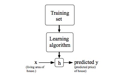
To describe the supervised learning problem slightly more formally, our goal is, given a training set, to learn a function h : X → Y so that h(x) is a “good” predictor for the corresponding value of y. For historical reasons, this function h is called a hypothesis(假设). Seen pictorially, the process is therefore like this:
Cost Function(代价函数)
We can measure the accuracy of our hypothesis function by using a cost function. This takes an average difference (actually a fancier version of an average) of all the results of the hypothesis with inputs from x's and the actual output y's.
This function is otherwise called the "Squared error function", or "Mean squared error"(MSE, 均方误差). The mean is halved(1/2) as a convenience for the computation of the gradient descent(梯度下降), as the derivative(导数) term of the square function will cancel out the 1/2 term.
calculus 微积分
Thus as a goal, we should try to minimize the cost function.
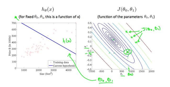
A contour(等高) plot is a graph that contains many contour lines. A contour line of a two variable function has a constant value at all points of the same line.
Taking any color and going along the 'circle', one would expect to get the same value of the cost function.
Plotting those values on our graph to the right seems to put our point in the center of the inner most 'circle'.
Parameter Learning
Gradient Descent(梯度下降)
So we have our hypothesis function and we have a way of measuring how well it fits into the data. Now we need to estimate the parameters in the hypothesis function. That's where gradient descent comes in.
Imagine that we graph our hypothesis function based on its fields θ0 and θ1(actually we are graphing the cost function as a function of the parameter estimates). We are not graphing x and y itself, but the parameter range of our hypothesis function and the cost resulting from selecting a particular set of parameters.
We put θ0 on the x axis and θ1 on the y axis, with the cost function on the vertical z axis. The points on our graph will be the result of the cost function using our hypothesis with those specific theta parameters. The graph below depicts such a setup.
We will know that we have succeeded when our cost function is at the very bottom of the pits in our graph, i.e. when its value is the minimum. The red arrows show the minimum points in the graph.
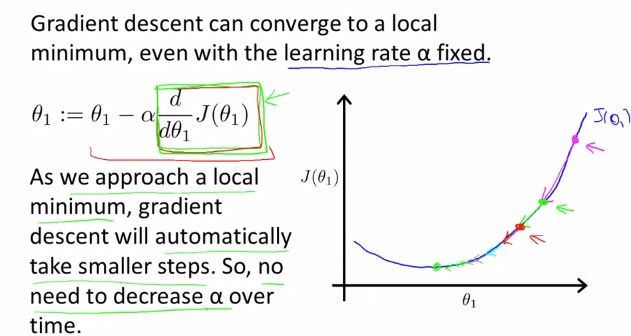
The way we do this is by taking the derivative(导数) (the tangential line to a function) of our cost function. The slope of the tangent is the derivative at that point and it will give us a direction to move towards. We make steps down the cost function in the direction with the steepest descent. The size of each step is determined by the parameter α, which is called the learning rate(学习率).
For example, the distance between each 'star' in the graph above represents a step determined by our parameter α. A smaller α would result in a smaller step and a larger α results in a larger step. The direction in which the step is taken is determined by the partial derivative(偏导数) of J(θ0, θ1). Depending on where one starts on the graph, one could end up at different points. The image above shows us two different starting points that end up in two different places.
The gradient descent algorithm is:
repeat until convergence(收敛):
where j=0,1 represents the feature index number.
At each iteration j, one should simultaneously update the parameters θ1,θ2,...,θn. Updating a specific parameter prior to calculating another one on the j^(th) iteration would yield to a wrong implementation.
Gradient Descent Intuition
we should adjust our parameter \alphaα to ensure that the gradient descent algorithm converges in a reasonable time. Failure to converge or too much time to obtain the minimum value imply that our step size is wrong.
If α is too small, gradient descent can be slow.
If α is too large, gradient descent can overshoot the minimum. It may fail to converge, or even diverge.
Gradient Descent For Linear Regression
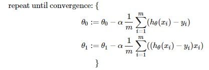
When specifically applied to the case of linear regression, a new form of the gradient descent equation can be derived. We can substitute our actual cost function and our actual hypothesis function and modify the equation to :
where m is the size of the training set, θ0 a constant that will be changing simultaneously with θ1 and x_{i}, y_{i} are values of the given training set (data).
So, this is simply gradient descent on the original cost function J. This method looks at every example in the entire training set on every step, and is called batch gradient descent. Note that, while gradient descent can be susceptible to local minima in general, the optimization problem we have posed here for linear regression has only one global, and no other local, optima; thus gradient descent always converges (assuming the learning rate α is not too large) to the global minimum. Indeed, J is a convex quadratic function(凸函数). Here is an example of gradient descent as it is run to minimize a quadratic function(二次函数).
The ellipses shown above are the contours of a quadratic function. Also shown is the trajectory taken by gradient descent, which was initialized at (48,30). The x’s in the figure (joined by straight lines) mark the successive values of θ that gradient descent went through as it converged to its minimum.
Linear Algebra Review
Matrices and Vectors (矩阵和向量)
Matrices are 2-dimensional arrays. A vector is a matrix with one column and many rows.
So vectors are a subset of matrices.
Addition and Scalar Multiplication
Addition and subtraction are element-wise, so you simply add or subtract each corresponding element:
In scalar multiplication, we simply multiply every element by the scalar value:
Matrix-Vector Multiplication
We map the column of the vector onto each row of the matrix, multiplying each element and summing the result.
The result is a vector. The number of columns of the matrix must equal the number of rows of the vector.
An m x n matrix multiplied by an n x 1 vector results in an m x 1 vector.
Matrix-Matrix Multiplication
We multiply two matrices by breaking it into several vector multiplications and concatenating the result.
Matrix Multiplication Properties
- Matrices are not commutative: A∗B≠B∗A
- Matrices are associative: (A∗B)∗C=A∗(B∗C)
The identity matrix, when multiplied by any matrix of the same dimensions, results in the original matrix. It's just like multiplying numbers by 1. The identity matrix simply has 1's on the diagonal (upper left to lower right diagonal) and 0's elsewhere.
Inverse and Transpose
The inverse of a matrix A is denoted A^(-1). Multiplying by the inverse results in the identity matrix.
A non square matrix does not have an inverse matrix. We can compute inverses of matrices in octave with the pinv(A) function and in Matlab with the inv(A) function. Matrices that don't have an inverse are singular or degenerate.
The transposition of a matrix is like rotating the matrix 90° in clockwise direction and then reversing it. We can compute transposition of matrices in matlab with the transpose(A) function or A':


