keras seq2seq_在Keras中建立具有Luong注意的Seq2Seq LSTM以进行时间序列预测

keras seq2seq

Do you want to try some other methods to solve your forecasting problem rather than traditional regression? There are many neural network architectures, which are frequently applied in NLP field, can be used for time series as well. In this article, we are going to build two Seq2Seq Models in Keras, the simple Seq2Seq LSTM Model, and the Seq2Seq LSTM Model with Luong Attention, and compare their forecasting accuracy.

您是否要尝试其他方法来解决预测问题，而不是传统回归方法？ 神经网络架构有很多，它们经常用于NLP领域，也可以用于时间序列。 在本文中，我们将在Keras中构建两个Seq2Seq模型，即简单的Seq2Seq LSTM模型和带有Luong Attention的Seq2Seq LSTM模型，并比较它们的预测准确性。

创建一些数据 (Create Some Data)

First of all, let’s create some time series data.

首先，让我们创建一些时间序列数据。

We’ve just created two sequences, x1 and x2, by combining sin waves, trend, and random noise. Next we will preprocess x1 and x2.

通过组合正弦波 ， 趋势和随机噪声 ，我们刚刚创建了两个序列x1和x2 。 接下来，我们将预处理x1和x2 。

预处理 (Preprocess)

1.将序列拆分为80％的训练集和20％的测试集 (1. Split sequences to 80% train set and 20% test set)

Since the sequence length is n_ = 1000, the first 800 data points will be used as our train data, while the rest will be used as our test data.

由于序列长度为n_ = 1000 ，因此前800个数据点将用作我们的火车数据，而其余的数据点将用作我们的测试数据。

2.去趋势 (2. Detrending)

It is not a must to detrend time series. However stationary time series will make model training much easier. There are many ways to detrend time series, such as taking difference of sequence with its lag1. Here for the simplicity, we assume the order of trend is known and we are just going to simply fit separate trend lines to x1 and x2, and then subtract the trend from the corresponding original sequence.

趋势曲线不是必须趋势。 但是，固定时间序列将使模型训练更加容易。 有许多种方法可以使时间序列趋于趋势，例如将序列与其lag1的差取值。 在这里，为简单起见，我们假定趋势的顺序是已知的，而我们只是简单地将单独的趋势线拟合到x1和x2 ，然后从相应的原始序列中减去趋势。

We will create index number of each position in the sequence, for easier detrending and trend recover.

我们将在序列中创建每个位置的索引号，以便于趋势下降和趋势恢复。

Here we will use np.polyfit to complete this small task. Note that only the first 800 data points are used to fit the trend lines, this is because we want to avoid data leak.

在这里，我们将使用np.polyfit完成此小任务。 请注意，只有前800个数据点用于拟合趋势线，这是因为我们要避免数据泄漏。

Based on the above values we got, we can now come up with the trend lines for x1 and x2.

基于上面得到的值，我们现在可以得出x1和x2的趋势线。

Let’s plot the trend lines together with x1 and x2, and check if they look good.

让我们将趋势线与x1和x2一起绘制，并检查它们是否看起来不错。

The above result looks fine, now we can deduct the trend.

以上结果看起来不错，现在我们可以推断趋势了。

After removing the trend, x1 and x2 become stationary.

消除趋势后，x1和x2变得平稳。

3.合并序列 (3. Combine sequences)

For easier preprocessing in next several steps, we can combine the sequences and their relevant information together into one array.

为了在接下来的几个步骤中更轻松地进行预处理，我们可以将序列及其相关信息组合到一个数组中。

In the combined array we created x_lbl:

在组合数组中，我们创建了x_lbl ：

• the first column is the detrended x1

  第一列是去趋势 x1

• the second column is the detrended x2

  第二列是去趋势 x2

• the third column is the index

  第三列是索引

• the fourth column is the label (1 for train set and 0 for test set)

  第四列是标签 (火车组为1，测试组为0)

4.归一化 (4. Normalize)

Normalisation can help model avoid favouring large features while ignoring very small features. Here we can just simply normalise x1 and x2 by dividing the corresponding maximum values in train set.

规范化可以帮助模型避免偏爱大型功能，而忽略非常小的功能。 在这里，我们可以简单地通过除以火车集合中的相应最大值来标准化x1和x2 。

Note that the above code only calculates maximum value of column 1 (detrended x1) and column 2 (detrended x2), the denominator of column 3 (index) and column 4 (label) are set to 1. This is because we do not input column 3 and column 4 into neural network, and hence no need to normalise them.

注意，上面的代码仅计算第1列(去趋势 x1 )和第2列(去趋势 x2 )的最大值，第3列( 索引 )和第4列( 标签 )的分母设置为1。这是因为我们没有输入第3列和第4列进入神经网络，因此无需对其进行标准化。

After normalisation, all the values are more or less within range from -1 to 1.

归一化后，所有值或多或少都在-1到1的范围内。

5.截断 (5. Truncate)

Next, we will cut sequence into smaller pieces by sliding an input window (length = 200 time steps) and an output window (length = 20 time steps), and put these samples in 3d numpy arrays.

接下来，我们将通过滑动一个输入窗口(长度= 200个时间步长)和一个输出窗口(长度= 20个时间步长)将序列切成更小的片段，并将这些样本放入3d numpy数组中。

The function truncate generates 3 arrays:

函数truncate生成3个数组：

• input to neural network X_in: it contains 781 samples, length of each sample is 200 time steps, and each sample contains 3 features: detrended and normalised x1, detrended and normalised x2, and original assigned data position index. Only the first 2 features will be used for training.

  输入到神经网络X_in ： 它包含781个样本，每个样本的长度为200个时间步长，并且每个样本都包含3个特征：去趋势化和归一化 x1 ，去趋势化和归一化 x2以及原始分配的数据位置索引 。 仅前两个功能将用于培训。

• target in neural network X_out: it contains 781 samples, length of each sample is 20 time steps, and each sample contains the same 3 features as in X_in. Only the first 2 features will be used as target, and the third feature will only be used to recover trend of the prediction.

  神经网络X_out中的目标： 它包含781个样本，每个样本的长度为20个时间步长，每个样本包含与X_in相同的3个特征。 仅前两个特征将用作目标，而第三个特征将仅用于恢复预测趋势。

• label lbl: 1 for train set and 0 for test set.

  标签lbl ：1代表火车，0代表测试。

Now the data is ready to be input into neural network!

现在可以将数据输入神经网络了！

模型1：简单的Seq2Seq LSTM模型 (Model 1: Simple Seq2Seq LSTM Model)

The above figure represents unfolded single layer of Seq2Seq LSTM model:

上图表示Seq2Seq LSTM模型的未折叠单层：

• The encoder LSTM cell: The value of each time step is input into the encoder LSTM cell together with previous cell state c and hidden state h, the process repeats until the last cell state c and hidden state h are generated.

  编码器LSTM单元 ：将每个时间步的值与先前的单元状态c和隐藏状态h一起输入到编码器LSTM单元中，重复此过程，直到生成最后的单元状态c和隐藏状态h 。

• The decoder LSTM cell: We use the last cell state c and hidden state h from the encoder as the initial states of the decoder LSTM cell. The last hidden state of encoder is also copied 20 times, and each copy is input into the decoder LSTM cell together with previous cell state c and hidden state h. The decoder outputs hidden state for all the 20 time steps, and these hidden states are connected to a dense layer to output the final result.

  解码器LSTM单元 ：我们使用编码器的最后一个单元状态c和隐藏状态h作为解码器LSTM单元的初始状态。 编码器的最后一个隐藏状态也被复制了20次，每个副本与先前的单元状态c和隐藏状态h一起输入到解码器LSTM单元中。 解码器输出所有20个时间步长的隐藏状态，并将这些隐藏状态连接到密集层以输出最终结果。

Set number of hidden layers:

设置隐藏层数：

The input layer

输入层

The encoder LSTM

编码器LSTM

We need to pay attention to 2 import parameters return_sequences and return_state, because they decide what LSTM returns.

我们需要注意2个导入参数return_sequences和return_state ，因为它们决定了LSTM返回什么。

• return_sequences=False, return_state=False: return the last hidden state: state_h

  return_sequences = False，return_state = False ：返回最后一个隐藏状态：state_h

• return_sequences=True, return_state=False: return stacked hidden states (num_timesteps * num_cells): one hidden state output for each input time step

  return_sequences = True，return_state = False ：返回堆叠的隐藏状态( num_timesteps * num_cells )：每个输入时间步长输出一个隐藏状态

• return_sequences=False, return_state=True: return 3 arrays: state_h, state_h, state_c

  return_sequences = False，return_state = True ：返回3个数组：state_h，state_h，state_c

• return_sequences=True, return_state=True: return 3 arrays: stacked hidden states, last state_h, last state_c

  return_sequences = True，return_state = True ：返回3个数组：堆叠的隐藏状态，最后一个state_h，最后一个state_c

For simple Seq2Seq model, we only need last state_h and last state_c.

对于简单的Seq2Seq模型，我们只需要last state_h和last state_c。

Batch normalisation is added because we want to avoid gradient explosion caused by the activation function ELU in the encoder.

添加批归一化是因为我们要避免编码器中激活函数ELU引起的梯度爆炸。

Next, we make 20 copies of the last hidden state of encoder and use them as input to the decoder. The last cell state and the last hidden state of the encoder are also used as the initial states of decoder.

接下来，我们复制编码器的最后一个隐藏状态的20个副本，并将其用作解码器的输入。 编码器的最后一个单元状态和最后一个隐藏状态也用作解码器的初始状态。

Then we put everything into the model, and compile it. Here we simply use MSE as the loss function and MAE as the evaluation metric. Note that we set clipnorm=1 for Adam optimiser. This is to normalise the gradient, so as to avoid gradient explosion during back propagation.

然后，我们将所有内容放入模型中并进行编译。 在这里，我们仅将MSE用作损失函数，将MAE用作评估指标。 请注意，我们为Adam optimiser设置了clipnorm = 1 。 这是为了规范化梯度，以避免在反向传播过程中梯度爆炸。

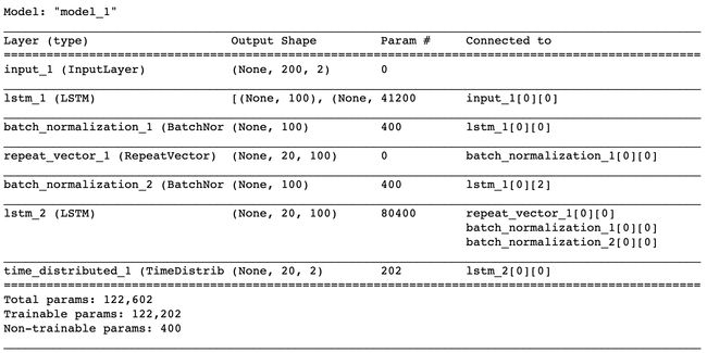
We can also plot the model:

我们还可以绘制模型：

The next step is training:

下一步是培训：

预测 (Prediction)

The model prediction as well as the true values are unnormalised:

模型预测以及真实值未归一化：

Then we combine the unnormalised outputs with their corresponding index, so that we can recover the trend.

然后，我们将未标准化的输出与其相应的索引结合起来，以便我们可以恢复趋势。

Next, we put all the outputs with recovered trend into a dictionary data_final.

接下来，我们将所有具有恢复趋势的输出放入字典data_final中 。

Just a quick check to see if the prediction value distribution is reasonable:

只需快速检查一下预测值分布是否合理：

The data distribution of prediction and true values are almost overlapped, so we are good.

预测值和真实值的数据分布几乎重叠，所以我们很好。

We can also plot MAE of all samples in time order, to see if there is clear pattern. The ideal situation is when line is random, otherwise it may indicate that the model is not sufficiently trained.

我们还可以按时间顺序绘制所有样本的MAE，以查看是否有清晰的图案。 理想的情况是线是随机的，否则可能表明模型未得到充分训练。

Based on the above plots, we can say that there are still certain periodical pattens in both train and test MAE. Training for more epochs may lead to better results.

根据以上图，我们可以说在训练和测试MAE中仍然有一定的周期性模式。 训练更多的时代可能会导致更好的结果。

Next we are going to check some random samples and see if the predicted lines and corresponding true lines are aligned.

接下来，我们将检查一些随机样本，看看预测线和相应的真实线是否对齐。

We can also check the nth prediction of each time step:

我们还可以检查每个时间步长的第n个预测：

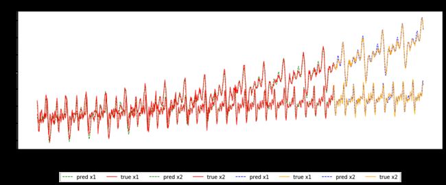
Take a closer look at the prediction on test set:

仔细查看测试集的预测：

模型2：具有Luong注意的Seq2Seq LSTM模型 (Model 2: Seq2Seq LSTM Model with Luong Attention)

https://blog.floydhub.com/attention-mechanism/ https://blog.floydhub.com/attention-mechanism/

One of the limitations of simple Seq2Seq model is: only the last state of encoder RNN is used as input to decoder RNN. If the sequence is very long, the encoder will tend to have much weaker memory about earlier time steps. Attention mechanism can solve this problem. An attention layer is going to assign proper weight to each hidden state output from encoder, and map them to output sequence.

简单Seq2Seq模型的局限性之一是：仅将编码器RNN的最后状态用作解码器RNN的输入。 如果序列很长，则编码器将在较早的时间步长上具有较弱的内存。 注意机制可以解决此问题。 注意层将为编码器输出的每个隐藏状态分配适当的权重，并将其映射到输出序列。

Next we will build Luong Attention on top of Model 1, and use Dot method to calculate alignment score.

接下来，我们将在模型1的顶部构建Luong Attention ，并使用Dot方法计算对齐分数。

The Input layer

输入层

It is the same as in Model 1:

与模型1相同：

The encoder LSTM

编码器LSTM

This is slightly different from Model 1: besides returning the last hidden state and the last cell state, we also need to return the stacked hidden states for alignment score calculation.

这与模型1稍有不同：除了返回最后一个隐藏状态和最后一个单元格状态，我们还需要返回堆叠的隐藏状态以计算比对分数 。

Next, we apply batch normalisation to avoid gradient explosion.

接下来，我们应用批量归一化以避免梯度爆炸。

The Decoder LSTM

解码器LSTM

Next, we repeat the last hidden state of encoder 20 times, and use them as input to decoder LSTM.

接下来，我们重复编码器的最后一个隐藏状态20次，并将其用作解码器LSTM的输入。

We also need to get the stacked hidden state of de decoder for alignment score calculation.

我们还需要获取解码器的堆叠隐藏状态以进行对齐分数计算。

Attention Layer

注意层

To build the attention layer, the first thing to do is to calculate the alignment score, and apply softmax activation function over it:

要构建关注层，首先要做的是计算对齐分数，并在其上应用softmax激活函数：

Then we can calculate the context vector, and also apply batch normalisation on top of it:

然后，我们可以计算上下文向量，并在其之上应用批处理规范化：

Now we concat the context vector and stacked hidden states of decoder, and use it as input to the last dense layer.

现在，我们结合上下文向量和解码器的堆叠隐藏状态，并将其用作最后一个密集层的输入。

Then we can compile the model. The parameters are the same as those in Model 1, for the sake of comparing the performance of the 2 models.

然后我们可以编译模型。 为了比较两个模型的性能，参数与模型1中的参数相同。

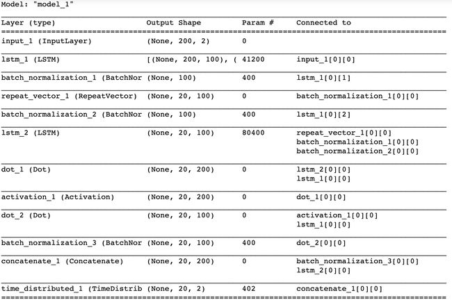
How data flow through the model:

数据如何流经模型：

The training and evaluation process is the same as illustrated in Model 1. After training for 100 epochs (the same number of training epochs as Model 1), we can evaluate the result.

培训和评估过程与模型1中所示的过程相同。 在训练了100个纪元后(与模型1相同的训练纪元数)，我们可以评估结果。

Below are the plots of sample MAE vs. sample order for train set and test set. Again, the model is not sufficiently trained since we can still see some periodical pattern. But for easier comparison of the 2 models, we are not going to train it more for now. Note that the overall MAE of both train set and test set are slightly improved compare to Model 1.

以下是火车集和测试集的样本MAE与样本顺序的图 。 同样，由于我们仍然可以看到一些周期性的模式，因此模型的训练不足。 但是为了更轻松地比较这两种模型，我们暂时不对其进行更多的培训。 请注意，与模型1相比，训练集和测试集的总体MAE都有所改善。

After adding the attention layer:

添加关注层后：

• MAE of train set decrease from 5.7851 to 5.7381
  火车的MAE从5.7851降低到5.7381
• MAE of test set decrease from 6.1495 to 5.9392
  测试集的MAE从6.1495降低到5.9392

Random sampling to check predicted line vs. true line:

随机抽样以检查预测线与真实线：

翻译自: https://levelup.gitconnected.com/building-seq2seq-lstm-with-luong-attention-in-keras-for-time-series-forecasting-1ee00958decb

keras seq2seq