Credit Fraud信用卡欺诈数据集，如何处理非平衡数据

简介

数据来源

数据集源自位于比利时布鲁塞尔ULB(Université Libre de Bruxelles) 的研究小组Worldline and the Machine Learning Group。数据集包含由欧洲持卡人于2013年9月使用信用卡在两天内发生的交易，284,807笔交易中有492笔被盗刷，正类（被盗刷）占所有交易的0.172％，数据集非常不平衡。它只包含作为PCA转换结果的数字输入变量。由于保密问题，特征V1，V2，… V28是使用PCA获得的主要组件，只有“交易时间”和“交易额”是原始特征。

可以从以下几个方面来探索数据集：

• 识别信用卡盗刷；
• 不平衡样本的处理方式 尝试不同的重采样是如何影响模型的效果
• 模型可以尝试Logistic回归、svm、决策树、XGBoost等进行预测

模型评价标准

由于样本的不平衡性与不平衡率，推荐使用Area Under the Precision-Recall Curve (AUPRC)来衡量准确率。注意，对于非平衡样本的分类，不推荐使用混淆矩阵（Confusion matrix）进行准确率评估，因为是没有意义的。所以可以在平衡样本后使用混淆矩阵评估准确率。

不平衡样本的处理

在这个数据集中，因为样本的极度不平衡，需要对样本进行分析，预处理之后再训练模型。本文介绍四种处理方式。

1. 不处理
2. 降采样
3. 过采样
4. SMOTE过采样

不平衡样本的分析

df = pd.read_csv('creditcard.csv')
df['Class'].value_counts()

0    284315
1       492
Name: Class, dtype: int64

在这个数据集中，Class = 0的样本数为 284315， 比例为 99.82%，Class =1 的样本数为492， 比例为 0.17%。如果不做任何处理，会导致很多分析失效。比如在分析特征和目标的关联性时，如果对数据不做处理，则有可能得不到任何有意义的结果。代码如下。

# set frac = 1 is to shuffle the samples
df = df.sample(frac = 1)
fraud_df = df.loc[df['Class'] == 1]
nofraud_df = df.loc[df['Class'] == 0][:492]

从数据集中按1：1的比例得到Class = 0 和 Class = 1 的训练数据，各492个。

normal_distributed_df = pd.concat([fraud_df, nofraud_df])
new_df = normal_distributed_df.sample(frac = 1, random_state = 42)
print(new_df['Class'].value_counts()/len(new_df))

1    0.5
0    0.5
Name: Class, dtype: float64

做correlation, 这里需要对两种情况进行分析，一个是极度非平衡的数据集，一个是降采样过后，比例为1：1的

## correlation, 这里需要对两种情况进行分析，一个是没有重采样的，一个是重采样，比例为1：1的
f,(ax1, ax2) = plt.subplots(2,1,figsize = [12,15])

corr = df.corr()
sns.heatmap(corr, cmap = 'coolwarm_r', annot_kws = {'size' : 20}, ax = ax1)
ax1.set_title('Imbalanced correlation matrix', fontsize = 14)

new_corr = new_df.corr()
sns.heatmap(new_corr,cmap = 'coolwarm_r', annot_kws = {'size' : 20}, ax = ax2)
ax2.set_title('Balanced correlation matrix', fontsize = 14)
plt.show()

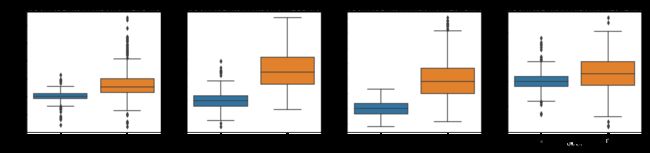
在imbalance的correlation中，几乎找不到正关系，但是在balanced中，V2,V4,V11,V19 是明显的正关系，V1，V3，V7，V10, V12, V14, V16, V17 是明显的负关系。 选择其中几种先看下正关系, V19关系最弱。

## 在imbalance的correlation中，几乎找不到正关系，但是在balanced中，
## V2,V4,V11,V19 是明显的正关系，V1，V3，V7，V10,V12,V14,V16,V17, 
## 选择其中几种先看下正关系, V19关系最弱
f, axes = plt.subplots(ncols = 4, figsize = [20,4])
sns.boxplot(x ='Class', y = 'V2', data = new_df, ax = axes[0])
axes[0].set_title('the positive correlation between V2 and y')

sns.boxplot(x ='Class', y = 'V4', data = new_df, ax = axes[1])
axes[1].set_title('the positive correlation between V4 and y')

sns.boxplot(x ='Class', y = 'V11', data = new_df, ax = axes[2])
axes[2].set_title('the positive correlation between V11 and y')

sns.boxplot(x ='Class', y = 'V19', data = new_df, ax = axes[3])
axes[3].set_title('the positive correlation between V19 and y')

plt.show()

f, axes = plt.subplots(ncols = 4, figsize = [20,4])

sns.boxplot(x = 'Class', y = 'V10', data = new_df, ax = axes[0])
axes[0].set_title('the negative correlation between V10 and class')
sns.boxplot(x = 'Class', y = 'V12', data = new_df, ax = axes[1])
axes[1].set_title('the negative correlation between V12 and class')
sns.boxplot(x = 'Class', y = 'V14', data = new_df, ax = axes[2])
axes[2].set_title('the negative correlation between V14 and class')
sns.boxplot(x = 'Class', y = 'V17', data = new_df, ax = axes[3])
axes[3].set_title('the negative correlation between V17 and class')
plt.show()

不处理样本

由上面的分析可知，如果对样本不处理，很有可能连基本的相关都得不到。其实在各种分类模型中，可以对不同的分类标签，设置不同的权重，通过这个权重能影响到损失函数。这里我先不对样本做处理，观察不同的权重对分类模型的性能的影响。

不设置权重

df = pd.read_csv('creditcard.csv')
X = df.drop(['Class'], axis = 1)
y = df['Class']
X_train, X_test, y_train, y_test = train_test_split(X,y,test_size = 0.2, random_state = 42)
X_train = X_train.values
X_test = X_test.values
y_train = y_train.values
y_test = y_test.values

from sklearn.model_selection import cross_val_score
from sklearn.linear_model import LogisticRegression
from sklearn.metrics import classification_report
lr_clf = LogisticRegression()
lr_clf.fit(X_train,y_train)
trainning_scores = cross_val_score(lr_clf, X_train,y_train, cv = 5)
print('logistic regression has a trainning score,', trainning_scores.mean()*100, '% accuracy')
## 这个只是accuracy ，不重要,关键是precision，recall，f1score和auc

logistic regression has a trainning score, 99.9043207946966 % accuracy

查看precision和recall

         -------- Classification Report --------
              precision    recall  f1-score   support

           0       1.00      1.00      1.00    284315
           1       0.86      0.60      0.71       492

    accuracy                           1.00    284807
   macro avg       0.93      0.80      0.85    284807
weighted avg       1.00      1.00      1.00    284807

设置权重，使用balanced

LogisticRegression()有一个参数class_weight，默认值为None，在本次实验中设置为 ‘balanced’。从结果来看，这个weight是根据class的比例来确定的，约为577。后面的实验会对class0 和class1 设置具体的权重，当class_weight = {0:1,1:500})时，分类器的性能与本次实验接近。

lr_model = LogisticRegression(class_weight = 'balanced')
lr_model.fit(x_train,y_train)
y_pred = lr_model.predict(x_test)
plotConfusionMatrixClassificationReport(y_test, y_pred, len_class0, len_class1)

             -------- Classification Report --------
              precision    recall  f1-score   support

           0       1.00      0.97      0.99     99511
           1       0.06      0.96      0.11       172

    accuracy                           0.97     99683
   macro avg       0.53      0.97      0.55     99683
weighted avg       1.00      0.97      0.98     99683

设置权重，使用不同的权重

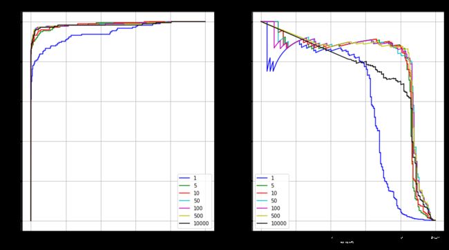
本次实验，对LogisticRegression()中的class_weight 设置具体的权重参数。其中class0的权重始终为1，而class1的权重为[1,5,10,50,100,500]。分析不同权重对分类器的影响。结果显示当class1的权重为5或者10的时候，precision和recall能取得比较好的平衡，当权重为50或500时，AUC(PR)较大。

for w in [1,5,10,50,100,500]:
    print('weight is {} for fraud class --'.format(w))
    lr_model = LogisticRegression(class_weight = {0:1,1:w})
    lr_model.fit(x_train,y_train)
    y_pred = lr_model.predict(x_test)
    plotConfusionMatrixClassificationReport(y_test, y_pred, len_class0, len_class1)
##
fig = plt.figure(figsize = [15,8]) 
ax1 = fig.add_subplot(1,2,1)
ax1.set_title('ROC CURVE')
ax1.set_xlim([-0.05,1.05])
ax1.set_ylim([-0.05,1.05])
ax1.set_xlabel('FPR')
ax1.set_ylabel('TPR')
plt.grid()

ax2 = fig.add_subplot(1,2,2)
ax2.set_title('PR CURVE')
ax2.set_xlim([-0.05, 1.05])
ax2.set_ylim([-0.05, 1.05])
ax2.set_xlabel('recall')
ax2.set_ylabel('precision')
plt.grid()
for w,k in zip([1,5,10,50,100,500,10000], 'bgrcmykw'):
    lr_model = LogisticRegression(class_weight = {0:1,1:w})
    lr_model.fit(x_train,y_train)
    y_pred = lr_model.predict(x_test)
    y_pred_prob = lr_model.predict_proba(x_test)[:,1]
    p,r,_ = precision_recall_curve(y_test, y_pred_prob)
    fpr, tpr,_ = roc_curve(y_test, y_pred_prob)
    precision = precision_score(y_test, y_pred)
    recall = recall_score(y_test, y_pred)
    roc_score = roc_auc_score(y_test, y_pred_prob)
    pr_score = auc(r,p)
    print('weight is {} for fraud class --'.format(w))
    print('the precision score is,',precision_score )
    print('the recall score is,',recall_score )
    print('the pr score is,', pr_score)
    ax1.plot(fpr, tpr, c=k, label = w)
    ax2.plot(r,p, c = k, label = w)
ax1.legend(loc = 'lower right')
ax2.legend(loc = 'lower left')
plt.show()

weight is 1 for fraud class --


         -------- Classification Report --------
              precision    recall  f1-score   support

           0       1.00      1.00      1.00     99511
           1       0.82      0.56      0.66       172

    accuracy                           1.00     99683
   macro avg       0.91      0.78      0.83     99683
weighted avg       1.00      1.00      1.00     99683

weight is 5 for fraud class --
         -------- Classification Report --------
              precision    recall  f1-score   support

           0       1.00      1.00      1.00     99511
           1       0.81      0.83      0.82       172

    accuracy                           1.00     99683
   macro avg       0.91      0.92      0.91     99683
weighted avg       1.00      1.00      1.00     99683

weight is 10 for fraud class --
         -------- Classification Report --------
              precision    recall  f1-score   support

           0       1.00      1.00      1.00     99511
           1       0.74      0.85      0.79       172

    accuracy                           1.00     99683
   macro avg       0.87      0.93      0.90     99683
weighted avg       1.00      1.00      1.00     99683

weight is 50 for fraud class --
         -------- Classification Report --------
              precision    recall  f1-score   support

           0       1.00      1.00      1.00     99511
           1       0.45      0.88      0.60       172

    accuracy                           1.00     99683
   macro avg       0.73      0.94      0.80     99683
weighted avg       1.00      1.00      1.00     99683

weight is 100 for fraud class --
         -------- Classification Report --------
              precision    recall  f1-score   support

           0       1.00      1.00      1.00     99511
           1       0.24      0.90      0.38       172

    accuracy                           0.99     99683
   macro avg       0.62      0.95      0.69     99683
weighted avg       1.00      0.99      1.00     99683

weight is 500 for fraud class --
      -------- Classification Report --------
              precision    recall  f1-score   support

           0       1.00      0.98      0.99     99511
           1       0.07      0.96      0.12       172

    accuracy                           0.98     99683
   macro avg       0.53      0.97      0.56     99683
weighted avg       1.00      0.98      0.99     99683

weight is 1 for fraud class --
the pr score is, 0.5836083385125052

weight is 5 for fraud class --
the pr score is, 0.7824530246938387

weight is 10 for fraud class --
the pr score is, 0.7866313311565967

weight is 50 for fraud class --
the pr score is, 0.8013701456084669

weight is 100 for fraud class --
the pr score is, 0.7971764777129003

weight is 500 for fraud class --
the pr score is, 0.8026288380720867

weight is 10000 for fraud class --
the pr score is, 0.7385516882490497

AUC(ROC) 与 AUC(PRC)对比

如上图所示，ROC曲线越凸向左上方向效果越好，PR曲线是右上凸效果越好。

当正负样本差距不大的情况下，ROC和PR的趋势是差不多的，但是当负样本很多的时候，两者就截然不同了，ROC效果依然看似很好，但是PR上反映效果一般。这个很好理解。在本次数据中，负样本远大于正样本。$$TPR=TP/(TP+FN)$$$$FPR=FP/(FP+TN)$$正样本很小，则TPR的分母很小，TPR会一直很大。负样本很大，则FPR的分母很大，此时即便FP数量够多，仍然对FPR影响较小，这样的话，ROC的结果会一直很好。

对于PR，Recall与TPR相同$$Recall=TP/(TP+FN)$$$$Precision=TP/(TP+FP)$$如果FP数量很大，因为TP数量会远小于FP，则对Precision指标会很差。因此对于正负样本区别较大的情况，PR更能准确反应模型性能。

总结

1. ROC曲线的特点是，当正负样本的分布发生变化时，ROC曲线的形状能够基本保持不变，而PR曲线回发生剧烈的变化。
2. 选择PR曲线还是ROC曲线是因实际问题而异的。ROC曲线能够更加稳定地反应模型本身地好坏。如果希望更多地看到模型在特定数据集上的表现，PR曲线更能够直观地反应其性能。

升采样

升采样SMOTE

SMOTE（Synthetic Minority Oversampling Technique），合成少数类过采样技术。它是基于随机过采样算法的一种改进方案，由于随机过采样采取简单复制样本的策略来增加少数类样本，这样容易产生模型过拟合的问题.

SMOTE算法的基本思想是对少数类样本进行分析并根据少数类样本人工合成新样本添加到数据集中,算法流程如下。

• 对于少数类中每一个样本$x$，以欧氏距离为标准计算它到少数类样本集中所有样本的距离，得到其k近邻。
• 根据样本不平衡比例设置一个采样比例以确定采样倍率N，对于每一个少数类样本$x$，从其k近邻中随机选择若干个样本，假设选择的近邻为$\tilde{x}$。
• 对于每一个随机选出的近邻$\tilde{x}$，分别与原样本按照如下的公式构建新的样本。类似一个线性插值的思想.
  $$x_{new}=x+rand(0,1)\ast (\tilde{x}-x)$$

from imblearn.over_sampling import SMOTE
os = SMOTE(random_state = 0)
df = pd.read_csv('creditcard.csv')
data_train_X,data_test_X,data_train_y,data_test_y=data_prepration(df)
columns = data_train_X.columns
os_data_X,os_data_y=os.fit_sample(data_train_X,data_train_y)
os_data_X = pd.DataFrame(data=os_data_X,columns=columns )
os_data_y= pd.DataFrame(data=os_data_y,columns=["Class"])

os_data_X['Normalized_Amount'] = StandardScaler().fit_transform(os_data_X['Amount'].values.reshape(-1, 1))
os_data_X.drop(['Time','Amount'],axis=1,inplace=True)
data_test_X['Normalized_Amount'] = StandardScaler().fit_transform(data_test_X['Amount'].values.reshape(-1, 1))
data_test_X.drop(["Time","Amount"],axis=1,inplace=True)
# Now start modeling
#clf= RandomForestClassifier(n_estimators=100)
# train data using oversampled data and predict for the test data
#model(clf,os_data_X,data_test_X,os_data_y,data_test_y)

_,(len_class0, len_class1) = np.unique(data_test_y, return_counts = True)
rndf_model = RandomForestClassifier(n_estimators = 100)
rndf_model.fit(os_data_X,os_data_y)
y_pred = rndf_model.predict(data_test_X)
plotConfusionMatrixClassificationReport(data_test_y, y_pred, len_class0, len_class1)

	-------- Classification Report --------
          precision    recall  f1-score   support

       0       1.00      1.00      1.00     85288
       1       0.88      0.86      0.87       155
  accuracy                            1.00     85443
  macro avg       0.94      0.93      0.93     85443	
  weighted avg    1.00      1.00      1.00     85443

the roc score is, 0.9690044131307659
the pr score is, 0.8758591483908675

XGBoost 建模

使用XGBoost模型做预测，其中参数如下

XGBC = xgb.XGBClassifier(
    gamma = 0.1,                      # Gamma指定了节点分裂所需的最小损失函数下降值，值越大，算法越保守。
    learning_rate = 0.3,              # 学习速率
    max_delta_step = 0,               # 限制每棵树权重改变的最大步长。0为没有限制，越大越保守。可用于样本不平衡的时候。
    max_depth = 5,                    # 树的最大深度
    min_child_weight = 6,             # 最小叶子节点样本权重和。低避免过拟合，太高导致欠拟合。
    missing = None,                   # 如果有缺失值则替换。默认 None 就是 np.nan
    n_estimators = 250,               # 树的数量
    nthread = 8,                      # 并行线程数量
    objective = 'binary:logistic',    # 指定学习任务和相应的学习目标或要使用的自定义目标函数
    #'objective':'multi:softprob',    # 定义学习任务及相应的学习目标
    #'objective':'reg:linear',        # 线性回归
    #'objective':'reg:logistic',      # 逻辑回归
    #'objective':'binary:logistic',   # 二分类的逻辑回归问题，输出为概率
    #'objective':'binary:logitraw',   # 二分类的逻辑回归问题，输出结果为 wTx，wTx指机器学习线性模型f(x)=wTx+b
    #'objective':'count:poisson'      # 计数问题的poisson回归，输出结果为poisson分布
    #'objective':'multi:softmax'      # 让XGBoost采用softmax目标函数处理多分类问题，同时需要设置参数num_class
    #'objective':'multi:softprob'     # 和softmax一样，但是输出的是ndata * nclass的向量，
                                      # 可以将该向量reshape成ndata行nclass列的矩阵。
                                      # 每行数据表示样本所属于每个类别的概率。
    reg_alpha = 1,                    # 权重的L1正则化项。默认1
    reg_lambda = 1,                   # 权重的L2正则化项。默认1
    scale_pos_weight = 500,           # 数字变大，会增加对少量诈骗样本的学习权重，这里500比较好
    seed = 0,                         # 随机种子
    silent = True,                    # 静默模式开启，不会输出任何信息
    subsample = 0.9,                  # 控制对于每棵树，随机采样的比例。减小会更加保守，避免过拟,过小会导致欠拟合。
    base_score = 0.5)                 # 所有实例的初始预测评分,全局偏差 

              precision    recall  f1-score   support

           0       1.00      1.00      1.00     99507
           1       0.91      0.82      0.87       176

    accuracy                           1.00     99683
   macro avg       0.96      0.91      0.93     99683
weighted avg       1.00      1.00      1.00     99683

the roc score is, 0.9772280753204206
the pr score is, 0.8462308516485526

参考链接

1. https://www.kaggle.com/lct14558/imbalanced-data-why-you-should-not-use-roc-curve
2. https://www.kaggle.com/janiobachmann/credit-fraud-dealing-with-imbalanced-datasets
3. XGBoost 与 信用卡诈骗数据集 三