深入Bert实战(Pytorch)----fine-Tuning 2

 

深入Bert实战(Pytorch)----fine-Tuning 2

https://www.bilibili.com/video/BV1K5411t7MD?p=5
https://www.youtube.com/channel/UCoRX98PLOsaN8PtekB9kWrw/videos
深入BERT实战(PyTorch) by ChrisMcCormickAI
这是ChrisMcCormickAI在油管bert，8集系列第三篇fine-Tuning的pytorch的讲解的代码，在油管视频下有cloab地址，如果不能的可以留下邮箱我全部看完整理后发给你。但是在fine-tuning最好还是在cloab上运行

 

文章目录

• 深入Bert实战(Pytorch)----fine-Tuning 2
• 4. Train Our Classification Model
• • 4.1. BertForSequenceClassification
  • 4.2. Optimizer & Learning Rate Scheduler
  • 4.3. 循环训练
• 5. 在测试集上的表现
• • 5.1. 数据准备
  • 5.2. 在测试集上评估
• 总结
• 附录
• • A1. Saving & Loading Fine-Tuned Model
• Revision History

 

---

4. Train Our Classification Model

4.1. BertForSequenceClassification

对于这个任务，我们首先要修改预训练的BERT模型以给出分类输出，然后在自己的数据集上继续训练模型，直到整个模型(端到端的模型)非常适合自己的任务。

值得庆幸的是，huggingface pytorch实现包含一组为各种NLP任务设计的接口。尽管这些接口都建立在训练好的BERT模型之上，但每个接口都有不同的顶层和输出类型，以适应它们特定的NLP任务。

这里是目前提供的fine-tuning列表

• BertModel
• BertForPreTraining
• BertForMaskedLM
• BertForNextSentencePrediction
• BertForSequenceClassification - The one we’ll use.
• BertForTokenClassification
• BertForQuestionAnswering

这里是transformer的文档here.

我们使用BertForSequenceClassification。这是普通的BERT模型，上面添加了一个用于分类的线性层，我们将使用它作为句子分类器。当我们输入数据时，整个预训练的BERT模型和额外的未训练的分类层是同时在这个任务上进行训练

好的，现在加载BERT！这里有几种不同的预训练模型，"bert-base-uncased"版本，仅有小写字母(“uncased”)相比于是较小的(“base” vs “large”)。

预训练的文档在from_pretrainedhere 定义了其它参数 here

from transformers import BertForSequenceClassification, AdamW, BertConfig

# Load BertForSequenceClassification, the pretrained BERT model with a single 
# linear classification layer on top. 
# 加载BertForSequenceClassification，预训练的模型+顶层单层线性分类层
model = BertForSequenceClassification.from_pretrained(
    "bert-base-uncased", # Use the 12-layer BERT model, with an uncased vocab.
    num_labels = 2, # The number of output labels--2 for binary classification.
                    # You can increase this for multi-class tasks.
    # 2分类问题，可以增加为多分类问题
    output_attentions = False, # Whether the model returns attentions weights.
    output_hidden_states = False, # Whether the model returns all hidden-states.
)

# Tell pytorch to run this model on the GPU.
model.cuda()

• 1
• 2
• 3
• 4
• 5
• 6
• 7
• 8
• 9
• 10
• 11
• 12
• 13
• 14
• 15
• 16

出于好奇，我们可以在这里按名称浏览所有的模型参数。
在下面的单元格中，我打印出了以下权重的名称和尺寸:

这里作者打印了所有层，总共有201层，也打印了权重和大小

1. The embedding layer.
2. The first of the twelve transformers.
3. The output layer.

# Get all of the model's parameters as a list of tuples.
params = list(model.named_parameters())

print('The BERT model has {:} different named parameters.\n'.format(len(params)))

print('==== Embedding Layer ====\n')

for p in params[0:5]:
    print("{:<55} {:>12}".format(p[0], str(tuple(p[1].size()))))

print('\n==== First Transformer ====\n')

for p in params[5:21]:
    print("{:<55} {:>12}".format(p[0], str(tuple(p[1].size()))))

print('\n==== Output Layer ====\n')

for p in params[-4:]:
    print("{:<55} {:>12}".format(p[0], str(tuple(p[1].size()))))

• 1
• 2
• 3
• 4
• 5
• 6
• 7
• 8
• 9
• 10
• 11
• 12
• 13
• 14
• 15
• 16
• 17
• 18
• 19

The BERT model has 201 different named parameters.

==== Embedding Layer ====

bert.embeddings.word_embeddings.weight                  (30522, 768)
bert.embeddings.position_embeddings.weight                (512, 768)
bert.embeddings.token_type_embeddings.weight                (2, 768)
bert.embeddings.LayerNorm.weight                              (768,)
bert.embeddings.LayerNorm.bias                                (768,)

==== First Transformer ====

bert.encoder.layer.0.attention.self.query.weight          (768, 768)
bert.encoder.layer.0.attention.self.query.bias                (768,)
bert.encoder.layer.0.attention.self.key.weight            (768, 768)
bert.encoder.layer.0.attention.self.key.bias                  (768,)
bert.encoder.layer.0.attention.self.value.weight          (768, 768)
bert.encoder.layer.0.attention.self.value.bias                (768,)
bert.encoder.layer.0.attention.output.dense.weight        (768, 768)
bert.encoder.layer.0.attention.output.dense.bias              (768,)
bert.encoder.layer.0.attention.output.LayerNorm.weight        (768,)
bert.encoder.layer.0.attention.output.LayerNorm.bias          (768,)
bert.encoder.layer.0.intermediate.dense.weight           (3072, 768)
bert.encoder.layer.0.intermediate.dense.bias                 (3072,)
bert.encoder.layer.0.output.dense.weight                 (768, 3072)
bert.encoder.layer.0.output.dense.bias                        (768,)
bert.encoder.layer.0.output.LayerNorm.weight                  (768,)
bert.encoder.layer.0.output.LayerNorm.bias                    (768,)

==== Output Layer ====

bert.pooler.dense.weight                                  (768, 768)
bert.pooler.dense.bias                                        (768,)
classifier.weight                                           (2, 768)
classifier.bias                                                 (2,)

• 1
• 2
• 3
• 4
• 5
• 6
• 7
• 8
• 9
• 10
• 11
• 12
• 13
• 14
• 15
• 16
• 17
• 18
• 19
• 20
• 21
• 22
• 23
• 24
• 25
• 26
• 27
• 28
• 29
• 30
• 31
• 32
• 33
• 34
• 35

4.2. Optimizer & Learning Rate Scheduler

现在我们已经加载了模型，我们需要从存储的模型中获取训练超参数。

为了进行微调，作者建议从以下值中进行选择。(从论文的注释 BERT paper):

• Batch size: 16, 32

• Learning rate (Adam): 5e-5, 3e-5, 2e-5
• Number of epochs: 2, 3, 4

作者选择的参数是：

• Batch size: 32 (set when creating our DataLoaders)
• Learning rate: 2e-5
• Epochs: 4 (we’ll see that this is probably too many…)

参数eps = 1e-8 是"a very small number to prevent any division by zero in the implementation"(from here)

您可以在run_glue.py中找到创建AdamW优化器的方法here.

# Note: AdamW is a class from the huggingface library (as opposed to pytorch) 
# AdamW是huggingface实现的类
# I believe the 'W' stands for 'Weight Decay fix"
optimizer = AdamW(model.parameters(),
                  lr = 2e-5, # args.learning_rate - default is 5e-5, our notebook had 2e-5
                  eps = 1e-8 # args.adam_epsilon  - default is 1e-8.
                )

• 1
• 2
• 3
• 4
• 5
• 6
• 7

from transformers import get_linear_schedule_with_warmup

# Number of training epochs. The BERT authors recommend between 2 and 4. 
# We chose to run for 4, but we'll see later that this may be over-fitting the
# training data.
epochs = 4

# Total number of training steps is [number of batches] x [number of epochs]. 
# (Note that this is not the same as the number of training samples).
total_steps = len(train_dataloader) * epochs    # 总共4 * 241批

# Create the learning rate scheduler.
scheduler = get_linear_schedule_with_warmup(optimizer, 
                                            num_warmup_steps = 0, # Default value in run_glue.py
                                            num_training_steps = total_steps)

• 1
• 2
• 3
• 4
• 5
• 6
• 7
• 8
• 9
• 10
• 11
• 12
• 13
• 14
• 15

4.3. 循环训练

下面是我们的训练循环。有很多事情要做，但从根本上来说，对于循环中的每一个过程，我们都有一个training阶段和一个validation阶段。

Thank you to Stas Bekman for contributing the insights and code for using validation loss to detect over-fitting!

Training:

• 打开我们的数据 inputs 和 labels
• 加载数据到GPU上
• 清除之前计算的梯度。
  • 在pytorch中，除非显式清除梯度，否则梯度默认累积(对于rnn之类的东西很有用)。
• Forward pass(通过网络输入数据)
• Backward pass 反向传播
• 告诉网络使用optimizer.step()更新参数
• 监控进度，跟踪变量

Evalution:

• 同训练过程一样，打开inputs 和 labels
• 加载数据到GPU上
• Forward pass(通过网络输入数据)
• 计算我们验证数据的损失，监控进度，跟踪变量

Pytorch向我们隐藏了所有详细的计算，但是我们已经对代码进行了注释，指出了每一行上发生的上述步骤。

定义一个计算精度的辅助函数。

import numpy as np

# Function to calculate the accuracy of our predictions vs labels
# 这个函数来计算预测值和labels的准确度
def flat_accuracy(preds, labels):
    pred_flat = np.argmax(preds, axis=1).flatten()    # 取出最大值对应的索引
    labels_flat = labels.flatten()
    return np.sum(pred_flat == labels_flat) / len(labels_flat)

• 1
• 2
• 3
• 4
• 5
• 6
• 7
• 8

格式化函数时间

import time
import datetime

def format_time(elapsed):
    '''
    Takes a time in seconds and returns a string hh:mm:ss
    '''
    # Round to the nearest second.    四舍五入
    elapsed_rounded = int(round((elapsed)))
    
    # Format as hh:mm:ss
    return str(datetime.timedelta(seconds=elapsed_rounded))

• 1
• 2
• 3
• 4
• 5
• 6
• 7
• 8
• 9
• 10
• 11
• 12

现在开始训练，这里要修改一部分代码，作者给的代码有个地方要做修改,参考run_glue.py

import random
import numpy as np

# This training code is based on the `run_glue.py` script here:
# https://github.com/huggingface/transformers/blob/5bfcd0485ece086ebcbed2d008813037968a9e58/examples/run_glue.py#L128

# Set the seed value all over the place to make this reproducible. 保证可重复性
seed_val = 42

random.seed(seed_val)
np.random.seed(seed_val)
torch.manual_seed(seed_val)
torch.cuda.manual_seed_all(seed_val)

# We'll store a number of quantities（保存如） such as training and validation loss, 
# validation accuracy, and timings.(训练loss, 验证loss, 验证准确率，训练时间)
training_stats = []

# Measure the total training time for the whole run. 总训练时间
total_t0 = time.time()

# For each epoch...
for epoch_i in range(0, epochs):
    
    # ========================================
    #               Training
    # ========================================
    # 对训练集进行一次完整的测试。
    print("")
    print('======== Epoch {:} / {:} ========'.format(epoch_i + 1, epochs))
    print('Training...')

    # Measure how long the training epoch takes.
    t0 = time.time()

    # Reset the total loss for this epoch.
    total_train_loss = 0

    # Put the model into training mode. Don't be mislead--the call to 
    # `train` just changes the *mode*, it doesn't *perform* the training.
    # 这里并不是执行的训练，而是，实例化启用 BatchNormalization 和 Dropout
    # `dropout` and `batchnorm` layers behave differently during training
    # vs. test (source: https://stackoverflow.com/questions/51433378/what-does-model-train-do-in-pytorch)
    model.train()

    # For each batch of training data...
    for step, batch in enumerate(train_dataloader):    # 共241个batches

        # Progress update every 40 batches.    40步打印一次
        if step % 40 == 0 and not step == 0:
            # Calculate elapsed time in minutes.
            elapsed = format_time(time.time() - t0)
            
            # Report progress.
            print('  Batch {:>5,}  of  {:>5,}.    Elapsed: {:}.'.format(step, len(train_dataloader), elapsed))
            # 例: Batch    40  of    241.    Elapsed: 0:00:08.

        # `batch` contains three pytorch tensors:
        #   [0]: input ids 
        #   [1]: attention masks
        #   [2]: labels 
        # 第一步的打开数据, 第二步 将数据放到GPU `to`方法
        b_input_ids = batch[0].to(device)
        b_input_mask = batch[1].to(device)
        b_labels = batch[2].to(device)

        # 在执行 backward pass 之前，始终清除任何先前计算的梯度。
        # PyTorch不会自动这样做，因为累积梯度“在训练rnn时很方便”。
        # (source: https://stackoverflow.com/questions/48001598/why-do-we-need-to-call-zero-grad-in-pytorch)
        model.zero_grad()    # 第三步，梯度清零      

        # 执行 forward pass (在此训练批次上对模型进行评估).
        # The documentation for this `model` function is here: 
        # https://huggingface.co/transformers/v2.2.0/model_doc/bert.html#transformers.BertForSequenceClassification
        # 它根据给定的参数和设置的标志返回不同数量的形参。
        # it returns the loss (because we provided labels) and the "logits"--the model outputs prior to activation.
        # 返回loss和"logits"--激活之前的模型输出。  model = BertForSequenceClassification
        output = model(b_input_ids, 
                             token_type_ids=None, 
                             attention_mask=b_input_mask, 
                             labels=b_labels)

        # 将所有批次的训练损失累积起来，这样我们就可以在最后计算平均损失。 
        # `loss` 是一个单个值的tensor; the `.item()` 函数将它转为一个python number
        loss, logits = output[:2]
        total_train_loss += loss.item()

        # 执行反向传播计算精度.
        loss.backward()

        # Clip the norm of the gradients to 1.0.
        # 梯度裁剪，防止梯度爆炸
        torch.nn.utils.clip_grad_norm_(model.parameters(), 1.0)

        # Update parameters and take a step using the computed gradient.
        # 更新参数，计算梯度
        # 优化器规定“update rule”——参数如何根据梯度、学习速率等进行修改。
        optimizer.step()

        # 更新学习率
        scheduler.step()

    # 计算平均loss
    avg_train_loss = total_train_loss / len(train_dataloader)            
    
    # 训练时间
    training_time = format_time(time.time() - t0)
    
    # 打印结果
    print("")
    print("  Average training loss: {0:.2f}".format(avg_train_loss))
    print("  Training epcoh took: {:}".format(training_time))
        
    # ========================================
    #               Validation
    # ========================================
    # 在验证集查看

    print("")
    print("Running Validation...")

    t0 = time.time()

    # 将模型置于评估模式 不使用BatchNormalization()和Dropout()
    model.eval()

    # 跟踪变量
    total_eval_accuracy = 0
    total_eval_loss = 0
    nb_eval_steps = 0

    # 在每个epoch上评估
    for batch in validation_dataloader:
        
        # `batch` contains three pytorch tensors:
        #   [0]: input ids 
        #   [1]: attention masks
        #   [2]: labels 
        b_input_ids = batch[0].to(device)
        b_input_mask = batch[1].to(device)
        b_labels = batch[2].to(device)
        
        # Tell pytorch not to bother with constructing the compute graph during
        # the forward pass, since this is only needed for backprop (training).
        with torch.no_grad():        

            # Forward pass, calculate logit predictions.
            # token_type_ids is the same as the "segment ids", which 
            # differentiates sentence 1 and 2 in 2-sentence tasks.
            # The documentation for this `model` function is here: 
            # https://huggingface.co/transformers/v2.2.0/model_doc/bert.html#transformers.BertForSequenceClassification
            # Get the "logits" output by the model. The "logits" are the output
            # values prior to applying an activation function like the softmax.
            (loss, logits) = model(b_input_ids, 
                                   token_type_ids=None, 
                                   attention_mask=b_input_mask,
                                   labels=b_labels)
            
        # 计算验证损失
        loss, logits = output[:2]
        total_eval_loss += loss.item()

        # Move logits and labels to CPU
        logits = logits.detach().cpu().numpy()
        label_ids = b_labels.to('cpu').numpy()

        # Calculate the accuracy for this batch of test sentences, and
        # accumulate it over all batches.
        total_eval_accuracy += flat_accuracy(logits, label_ids)
        

    # 返回验证结果
    avg_val_accuracy = total_eval_accuracy / len(validation_dataloader)
    print("  Accuracy: {0:.2f}".format(avg_val_accuracy))

    # 计算平均复杂度
    avg_val_loss = total_eval_loss / len(validation_dataloader)
    
    # 时间
    validation_time = format_time(time.time() - t0)
    
    print("  Validation Loss: {0:.2f}".format(avg_val_loss))
    print("  Validation took: {:}".format(validation_time))

    # 记录这个epoch的所有统计数据。 方便后面可视化
    training_stats.append(
        {
            'epoch': epoch_i + 1,
            'Training Loss': avg_train_loss,
            'Valid. Loss': avg_val_loss,
            'Valid. Accur.': avg_val_accuracy,
            'Training Time': training_time,
            'Validation Time': validation_time
        }
    )

print("")
print("Training complete!")

print("Total training took {:} (h:mm:ss)".format(format_time(time.time()-total_t0)))

• 1
• 2
• 3
• 4
• 5
• 6
• 7
• 8
• 9
• 10
• 11
• 12
• 13
• 14
• 15
• 16
• 17
• 18
• 19
• 20
• 21
• 22
• 23
• 24
• 25
• 26
• 27
• 28
• 29
• 30
• 31
• 32
• 33
• 34
• 35
• 36
• 37
• 38
• 39
• 40
• 41
• 42
• 43
• 44
• 45
• 46
• 47
• 48
• 49
• 50
• 51
• 52
• 53
• 54
• 55
• 56
• 57
• 58
• 59
• 60
• 61
• 62
• 63
• 64
• 65
• 66
• 67
• 68
• 69
• 70
• 71
• 72
• 73
• 74
• 75
• 76
• 77
• 78
• 79
• 80
• 81
• 82
• 83
• 84
• 85
• 86
• 87
• 88
• 89
• 90
• 91
• 92
• 93
• 94
• 95
• 96
• 97
• 98
• 99
• 100
• 101
• 102
• 103
• 104
• 105
• 106
• 107
• 108
• 109
• 110
• 111
• 112
• 113
• 114
• 115
• 116
• 117
• 118
• 119
• 120
• 121
• 122
• 123
• 124
• 125
• 126
• 127
• 128
• 129
• 130
• 131
• 132
• 133
• 134
• 135
• 136
• 137
• 138
• 139
• 140
• 141
• 142
• 143
• 144
• 145
• 146
• 147
• 148
• 149
• 150
• 151
• 152
• 153
• 154
• 155
• 156
• 157
• 158
• 159
• 160
• 161
• 162
• 163
• 164
• 165
• 166
• 167
• 168
• 169
• 170
• 171
• 172
• 173
• 174
• 175
• 176
• 177
• 178
• 179
• 180
• 181
• 182
• 183
• 184
• 185
• 186
• 187
• 188
• 189
• 190
• 191
• 192
• 193
• 194
• 195
• 196
• 197
• 198
• 199
• 200

让我们来看看训练过程的总结。

import pandas as pd

# 显示浮点数小数点后两位。
pd.set_option('precision', 2)

# 从训练统计数据里，创建一个 DataFrame
df_stats = pd.DataFrame(data=training_stats)

# 用'epoch'行坐标
df_stats = df_stats.set_index('epoch')

# A hack to force the column headers to wrap.
#df = df.style.set_table_styles([dict(selector="th",props=[('max-width', '70px')])])

# Display the table.
df_stats

• 1
• 2
• 3
• 4
• 5
• 6
• 7
• 8
• 9
• 10
• 11
• 12
• 13
• 14
• 15
• 16

Training Loss	Valid. Loss	Valid. Accur.	Training Time	Validation Time epoch
1	0.50	0.45	0.80	0:00:51
2	0.32	0.46	0.81	0:00:51
3	0.22	0.49	0.82	0:00:51
4	0.16	0.55	0.82	0:00:51

这里我跑这代码train loss没有下降，反而上升了，有了解这个问题的大大，麻烦请留言指教下

请注意，当训练损失随着时间的推移而下降时，验证损失却在增加!这表明我们训练模型的时间太长了，它对训练数据过于拟合。

(作为参考，我们使用了7,695个训练样本和856个验证样本)。

验证损失是比精度更精确的度量，因为有了精度，我们不关心确切的输出值，而只关心它落在阈值的哪一边。

如果我们预测的是正确的答案，但缺乏信心，那么验证损失将捕捉到这一点，而准确性则不会。

import matplotlib.pyplot as plt
% matplotlib inline

import seaborn as sns

# Use plot styling from seaborn.
sns.set(style='darkgrid')

# Increase the plot size and font size.
sns.set(font_scale=1.5)
plt.rcParams["figure.figsize"] = (12,6)

# 绘制学习曲线
plt.plot(df_stats['Training Loss'], 'b-o', label="Training")
plt.plot(df_stats['Valid. Loss'], 'g-o', label="Validation")

# Label the plot.
plt.title("Training & Validation Loss")
plt.xlabel("Epoch")
plt.ylabel("Loss")
plt.legend()
plt.xticks([1, 2, 3, 4])

plt.show()

• 1
• 2
• 3
• 4
• 5
• 6
• 7
• 8
• 9
• 10
• 11
• 12
• 13
• 14
• 15
• 16
• 17
• 18
• 19
• 20
• 21
• 22
• 23
• 24

5. 在测试集上的表现

现在，我们将加载holdout数据集并准备输入，就像我们对训练集所做的那样。然后，我们将使用Matthew’s correlation coefficient评估预测，因为这是更广泛的NLP社区用于评估CoLA性能的指标。在这个指标下，+1是最好的分数，-1是最差的分数。通过这种方式，我们可以看到针对这个特定任务的先进模型的性能如何。

5.1. 数据准备

我们需要应用与训练数据相同的所有步骤来准备测试数据集。

import pandas as pd

# 加载数据
df = pd.read_csv("./cola_public/raw/out_of_domain_dev.tsv", delimiter='\t', header=None, names=['sentence_source', 'label', 'label_notes', 'sentence'])

# 显示句子数量
print('Number of test sentences: {:,}\n'.format(df.shape[0]))

# 创建句子和标签列表
sentences = df.sentence.values
labels = df.label.values

# Tokenize 
input_ids = []
attention_masks = []

# For every sentence...
for sent in sentences:
    # `encode_plus` will:
    #   (1) Tokenize the sentence.
    #   (2) 添加 `[CLS]` token 到开始
    #   (3) 添加 `[SEP]` token 到结束
    #   (4) 映射tokens 到 IDs.
    #   (5) 填充或截断句子到`max_length`
    #   (6) Create attention masks for [PAD] tokens.
    encoded_dict = tokenizer.encode_plus(
                        sent,                      # 对句子做encode.
                        add_special_tokens = True, # Add '[CLS]' and '[SEP]'
                        max_length = 64,           # Pad & truncate all sentences.
                        pad_to_max_length = True,
                        return_attention_mask = True,   # Construct attn. masks.
                        return_tensors = 'pt',     # Return pytorch tensors.
                   )
    
    # 将已编码的句子添加到列表中。  
    input_ids.append(encoded_dict['input_ids'])
    
    # 以及它的注意力掩码(简单地区分填充和非填充)。
    attention_masks.append(encoded_dict['attention_mask'])

# Convert the lists into tensors.
input_ids = torch.cat(input_ids, dim=0)
attention_masks = torch.cat(attention_masks, dim=0)
labels = torch.tensor(labels)

# Set the batch size.  
batch_size = 32  

# Create the DataLoader.
prediction_data = TensorDataset(input_ids, attention_masks, labels)
prediction_sampler = SequentialSampler(prediction_data)
prediction_dataloader = DataLoader(prediction_data, sampler=prediction_sampler, batch_size=batch_size)

• 1
• 2
• 3
• 4
• 5
• 6
• 7
• 8
• 9
• 10
• 11
• 12
• 13
• 14
• 15
• 16
• 17
• 18
• 19
• 20
• 21
• 22
• 23
• 24
• 25
• 26
• 27
• 28
• 29
• 30
• 31
• 32
• 33
• 34
• 35
• 36
• 37
• 38
• 39
• 40
• 41
• 42
• 43
• 44
• 45
• 46
• 47
• 48
• 49
• 50
• 51
• 52

Number of test sentences: 516

5.2. 在测试集上评估

准备好测试集之后，我们可以应用我们的微调模型来生成测试集的预测。

# Prediction on test set

print('Predicting labels for {:,} test sentences...'.format(len(input_ids)))

# 在测试模型
model.eval()

# 跟踪变量 
predictions , true_labels = [], []

# Predict 
for batch in prediction_dataloader:
  # Add batch to GPU
  batch = tuple(t.to(device) for t in batch)
  
  # Unpack the inputs from our dataloader
  b_input_ids, b_input_mask, b_labels = batch
  
  # 不让模型计算或存储梯度，节省内存和加速预测
  with torch.no_grad():
      # Forward pass, calculate logit predictions
      outputs = model(b_input_ids, token_type_ids=None, 
                      attention_mask=b_input_mask)

  logits = outputs[0]

  # Move logits and labels to CPU
  logits = logits.detach().cpu().numpy()
  label_ids = b_labels.to('cpu').numpy()
  
  # Store predictions and true labels
  predictions.append(logits)
  true_labels.append(label_ids)

print('    DONE.')

• 1
• 2
• 3
• 4
• 5
• 6
• 7
• 8
• 9
• 10
• 11
• 12
• 13
• 14
• 15
• 16
• 17
• 18
• 19
• 20
• 21
• 22
• 23
• 24
• 25
• 26
• 27
• 28
• 29
• 30
• 31
• 32
• 33
• 34
• 35

CoLA基准的精度是用“Matthews correlation coefficient”来测量的。(MCC)。

我们在这里使用MCC是因为类是不平衡的:

print('Positive samples: %d of %d (%.2f%%)' % (df.label.sum(), len(df.label), (df.label.sum() / len(df.label) * 100.0)))

• 1

Positive samples: 354 of 516 (68.60%)

# 计算相关系数
from sklearn.metrics import matthews_corrcoef

matthews_set = []

# 使用Matthew相关系数对每个测试批进行评估
print('Calculating Matthews Corr. Coef. for each batch...')

# For each input batch...
for i in range(len(true_labels)):
  
  # 这个批处理的预测是一个2列的ndarray(一个列是“0”，一个列是“1”)。 
  # 选择值最高的label，并将其转换为0和1的列表。
  pred_labels_i = np.argmax(predictions[i], axis=1).flatten()
  
  # Calculate and store the coef for this batch.  
  matthews = matthews_corrcoef(true_labels[i], pred_labels_i)                
  matthews_set.append(matthews)

• 1
• 2
• 3
• 4
• 5
• 6
• 7
• 8
• 9
• 10
• 11
• 12
• 13
• 14
• 15
• 16
• 17
• 18

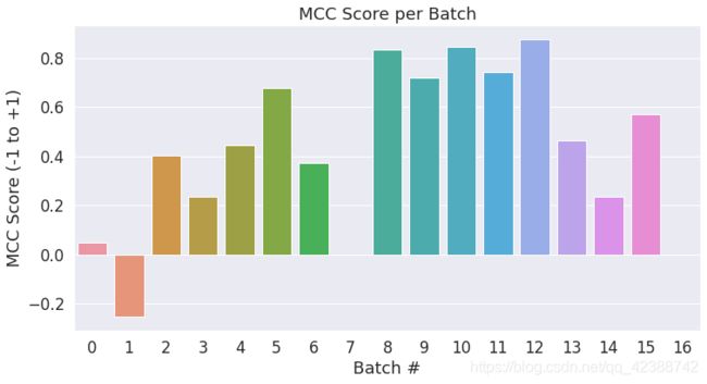
最终的分数将基于整个测试集，但是让我们看一下单个批次的分数，以了解批次之间度量的可变性。

每批有32个句子，除了最后一批只有(516% 32)= 4个测试句子。

创建一个柱状图，显示每批测试样品的MCC分数。

ax = sns.barplot(x=list(range(len(matthews_set))), y=matthews_set, ci=None)

plt.title('MCC Score per Batch')
plt.ylabel('MCC Score (-1 to +1)')
plt.xlabel('Batch #')

plt.show()

• 1
• 2
• 3
• 4
• 5
• 6
• 7

现在我们将合并所有批次的结果并计算我们最终的MCC分数。

# 合并所有批次的结果。
flat_predictions = np.concatenate(predictions, axis=0)

# 对于每个样本，选择得分较高的标签(0或1)。
flat_predictions = np.argmax(flat_predictions, axis=1).flatten()

# 将每个批次的正确标签组合成一个单独的列表。
flat_true_labels = np.concatenate(true_labels, axis=0)

# Calculate the MCC
mcc = matthews_corrcoef(flat_true_labels, flat_predictions)

print('Total MCC: %.3f' % mcc)

• 1
• 2
• 3
• 4
• 5
• 6
• 7
• 8
• 9
• 10
• 11
• 12
• 13

在大约半个小时的时间里，我们没有做任何超参数的调整(learning rate, epochs, batch size, ADAM properties属性等)，我们就获得了一个很好的分数。

为了使分数最大化，我们应该删除“验证集”(我们用来帮助确定要训练多少个纪元)，并在整个训练集上训练。

库将基准测试此处的预期精度文档为“49.23”。

官方排行 here.

请注意(由于数据集的大小较小?)在不同的运行中，精度可能会有很大的变化。

总结

这篇文章演示了使用预先训练好的BERT模型，不管你感兴趣的是什么特定的NLP任务，你都可以使用pytorch接口，用最少的努力和训练时间，快速有效地创建一个高质量的模型。

附录

A1. Saving & Loading Fine-Tuned Model

(取自’ run_glue。py 'here)将模型和标记器写入磁盘。

import os

# 保存best-practices:如果您使用模型的默认名称，您可以使用from_pretraining()重新加载它
# Saving best-practices: if you use defaults names for the model, you can reload it using from_pretrained()

output_dir = './model_save/'

# 如果需要，创建输出目录
if not os.path.exists(output_dir):
    os.makedirs(output_dir)

print("Saving model to %s" % output_dir)

# 使用`save_pretrained()`保存训练过的模型、配置和标记器。
# 用`from_pretrained()`重新加载模型。
model_to_save = model.module if hasattr(model, 'module') else model  # 注意distributed/parallel training
model_to_save.save_pretrained(output_dir)
tokenizer.save_pretrained(output_dir)

# Good practice: 保存训练好的模型于模型参数
# torch.save(args, os.path.join(output_dir, 'training_args.bin'))

• 1
• 2
• 3
• 4
• 5
• 6
• 7
• 8
• 9
• 10
• 11
• 12
• 13
• 14
• 15
• 16
• 17
• 18
• 19
• 20
• 21
• 22

Revision History

Version 3 - Mar 18th, 2020 - (current)

• Simplified the tokenization and input formatting (for both training and test) by leveraging the tokenizer.encode_plus function.
  encode_plus handles padding and creates the attention masks for us.
• Improved explanation of attention masks.
• Switched to using torch.utils.data.random_split for creating the training-validation split.
• Added a summary table of the training statistics (validation loss, time per epoch, etc.).
• Added validation loss to the learning curve plot, so we can see if we’re overfitting.
  • Thank you to Stas Bekman for contributing this!
• Displayed the per-batch MCC as a bar plot.

Version 2 - Dec 20th, 2019 - link

• huggingface renamed their library to transformers.
• Updated the notebook to use the transformers library.

Version 1 - July 22nd, 2019

• Initial version.