Python数据分析之pandas库的使用详解

本篇文章所依据是蚂蚁学Python作者讲解所写，且已征求作者的同意，内容基本都是视频中所讲的内容。视频满满的全是干货，也可一边看视频一边配合着本篇文章。

作者的公众号：蚂蚁学Python 视频地址

当然作者也提供了代码和课件，在视频的评论区就能找到。本篇文章的代码也可以参考，如有需要，可以私聊发送。
本篇文章有两章没有写完，之后会补充完整。

一、前言

Numpy能够帮助我们处理数值型数据，但这是远远不够的，很多时候，我们需要处理的数据中不仅仅时数值型数据，还有字符串，时间序列等等。所以Numpy能够帮助我们处理数值，但是pandas除了梳理数值之外（基于Numpy），还能构帮助我们处理其他类型的数据。

二、什么是pandas

一个开源的python类库：用于数据分析、数据处理、数据可视化

• 特点：高性能，容易使用的数据结构，容易使用的数据分析工具

三、pandas安装

pip install pandas

四、pandas的常用数据类型

4.1 series：表示一维，带标签数组，一行或一列

4.1.1创建series

示例代码：

import pandas as pd

# 创建一个Series
t = pd.Series([1, 2, 'p', 3, 'a'])
# 输出的结果，左侧为索引，右侧为数据
print(t)
输出结果：
0    1
1    2
2    p
3    3
4    a
dtype: object

4.1.2 打印索引值

通过index则可以打印出索引值
示例代码：

import pandas as pd

# 创建一个Series
t = pd.Series([1, 2, 'p', 3, 'a'])
# 打印索引值
print(t.index)
输出结果：
RangeIndex(start=0, stop=5, step=1)

4.1.3 打印数据值

通过values可以获得我们数据值
示例代码：

import pandas as pd

# 创建一个Series
t = pd.Series([1, 2, 'p', 3, 'a'])
# 打印数据值
print(t.values)
输出结果：
[1 2 'p' 3 'a']

4.1.3 创建一个具有标签索引的series

指定index则会创建一个具有标签索引的serie
示例代码：

import pandas as pd

#  创建一个具有标签索引的series
f = pd.Series([1, 2, 'p', 3, 'a'], index=[11, 22, 33, 44, 55])
print(f)
输出结果：
11    1
22    2
33    p
44    3
55    a
dtype: object

4.1.4 使用python字典创建series

示例代码：

import pandas as pd

data = {"name": "tom", "gender": "man", "age": 18}
g = pd.Series(data)
print(g)
输出结果：
name      tom
gender    man
age        18
dtype: object

4.1.5 根据索引值查询数据

• 查询单个数据与字典查询数据类似方法
  示例代码：

import pandas as pd

f = pd.Series([1, 2, 'p', 3, 'a'], index=[11, 22, 33, 44, 55])
# 使用索引值查询数据
print(f[11])
输出结果：
1

• 查询多个数据
  示例代码：

import pandas as pd

f = pd.Series([1, 2, 'p', 3, 'a'], index=[11, 22, 33, 44, 55])
# 使用索引值查询多个数据
print(f[[11, 22]])
输出结果：
11    1
22    2
dtype: object

4.2 DataFrame：表示二维，多行多列

DataFrame是一个表格型的数据结构

• 每列可以是不同值的类型（数值，字符串，布尔值等）
• 既有行索引index，也有列索引columns
• 可以被看做由Series组成的字典

4.2.1DataFrame创建

4.2.1.1 根据字典创建DataFrame

示例代码：

import pandas as pd

# 根据字典创建DataFrame
data = {
    "name": ["Tom", "rose", "json"],
    "age": [12, 21, 23],
    "gender": ["man", "woman", "man"]
}
# 调用DataFrame方法
df = pd.DataFrame(data)
print(df)
输出结果：
   name  age gender
0   Tom   12    man
1  rose   21  woman
2  json   23    man

4.2.1.2 查看类型

调用dtypes方法可查看我们的数据每一列的数据类型
示例代码：

import pandas as pd

# 根据字典创建DataFrame
data = {
    "name": ["Tom", "rose", "json"],
    "age": [12, 21, 23],
    "gender": ["man", "woman", "man"]
}
# 调用DataFrame方法
df = pd.DataFrame(data)
print(df.dtypes)
输出如果：
name      object
age        int64
gender    object
dtype: object

4.2.1.3 查看列索引

通过columns方法可以查看我们数据的列索引
示例代码：

import pandas as pd

# 根据字典创建DataFrame
data = {
    "name": ["Tom", "rose", "json"],
    "age": [12, 21, 23],
    "gender": ["man", "woman", "man"]
}
# 调用DataFrame方法
df = pd.DataFrame(data)
print(df.columns)
输出结果：
Index(['name', 'age', 'gender'], dtype='object')

4.2.1.4 查看行索引

通过index方法可以查看我们数据的列索引

import pandas as pd

# 根据字典创建DataFrame
data = {
    "name": ["Tom", "rose", "json"],
    "age": [12, 21, 23],
    "gender": ["man", "woman", "man"]
}
# 调用DataFrame方法
df = pd.DataFrame(data)
print(df.index)
输出结果：
RangeIndex(start=0, stop=3, step=1)

4.2.2 从DataFrame中查询Series

• 如果只查询一行、一列、返回的是pd.Series
• 如果查询多行、多列，返回的是pd.DataFrame

4.2.2.1 查询一列，结果是一个pd.Series

示例代码：

import pandas as pd

# 根据字典创建DataFrame
data = {
    "name": ["Tom", "rose", "json"],
    "age": [12, 21, 23],
    "gender": ["man", "woman", "man"]
}
# 调用DataFrame方法
df = pd.DataFrame(data)
print(df)
输出结果：
   name  age gender
0   Tom   12    man
1  rose   21  woman
2  json   23    man
print(df["name"])
输出结果：
0     Tom
1    rose
2    json
Name: name, dtype: object

4.2.2.2 查询多列，结果是一个pd.DataFrame

示例代码：

import pandas as pd

# 根据字典创建DataFrame
data = {
    "name": ["Tom", "rose", "json"],
    "age": [12, 21, 23],
    "gender": ["man", "woman", "man"]
}
# 调用DataFrame方法
df = pd.DataFrame(data)
print(df)
输出结果：
   name  age gender
0   Tom   12    man
1  rose   21  woman
2  json   23    man
print(df[["name","age"]])
输出结果：
   name  age
0   Tom   12
1  rose   21
2  json   23
print(type(df[["name","age"]]))
输出结果“
<class 'pandas.core.frame.DataFrame'>

4.2.2.3 查询一行，结果是一个pd.Series

示例代码：

import pandas as pd

# 根据字典创建DataFrame
data = {
    "name": ["Tom", "rose", "json"],
    "age": [12, 21, 23],
    "gender": ["man", "woman", "man"]
}
# 调用DataFrame方法
df = pd.DataFrame(data)
print(df)
输出结果：
   name  age gender
0   Tom   12    man
1  rose   21  woman
2  json   23    man
# 查询一行
print(df.loc[1])
输出结果：
name       rose
age          21
gender    woman
Name: 1, dtype: object

4.2.2.4 查询多行，结果是一个pd.DataFrame

示例代码：

import pandas as pd

# 根据字典创建DataFrame
data = {
    "name": ["Tom", "rose", "json"],
    "age": [12, 21, 23],
    "gender": ["man", "woman", "man"]
}
# 调用DataFrame方法
df = pd.DataFrame(data)
print(df)
输出结果：
   name  age gender
0   Tom   12    man
1  rose   21  woman
2  json   23    man
# 查询多行
print(df.loc[0:1])
输出结果：
   name  age gender
0   Tom   12    man
1  rose   21  woman

五、数据的读取

5.1 常用数据格式读取方式

5.2 pandas读取csv文件

pandas读取csv文件通过调用read_csv即可。

5.2.1 读取整篇文件

示例代码：

import pandas as pd

t = pd.read_csv("proxy.csv")
print(t)

5.2.2 pandas读取前几行

通过head()方法，可以读取csv文件中的前几行内容。
示例代码：

import pandas as pd

t = pd.read_csv("proxy.csv")
print(t.head())

输出结果：

5.2.3 pandas查看数据的形状，返回（行数、列数）

通过.shape方法，可查看csv文件的形状。
示例代码：

import pandas as pd

t = pd.read_csv("proxy.csv")
print(t.shape)
输出结果：
(9999, 1)

5.2.4 pandas查看列名列表

import pandas as pd

t = pd.read_csv("proxy.csv")
# 查看列名列表
print(t.columns)
输出结果：
Index(['http://106.122.205.38:8118'], dtype='object')

5.2.5 pandas查看索引列

import pandas as pd

t = pd.read_csv("proxy.csv")
# 查看索引列
print(t.index)
输出结果：
RangeIndex(start=0, stop=9999, step=1)

5.2.6 pandas查看数据类型

import pandas as pd

t = pd.read_csv("proxy.csv")
# 查看数据类型
print(t.dtypes)
输出结果：
http://106.122.205.38:8118    object
dtype: object

5.3 pandas读取txt文件

5.4 pandas读取excel文件

示例代码：

import pandas as pd

f = pd.read_excel("pandas数据读取.xlsx")
print(f)

输出结果：

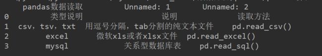
5.5 pandas读取mysql文件

六、数据的查询

6.1 pandas查询数据的几种方式

• df.loc方法，根据行、列的标签值查询
• df.iloc方法，根据行、列的数字位置进行查询
• df.where方法
• df.query方法
  .loc方法既能查询，又能覆盖写入

6.2 pandas使用loc查询数据

• 使用单个标签值查询数据
• 使用值列表批量查询
• 使用数值区间进行范围查询
• 使用条件表达式查询
• 调用函数查询
  注意：以上查询方法，既适合行也适合列。注意观察降维DataFrame > Series > 值

6.2.1 使用单个Label值查询数据

行或者列，都可以只传入单个值，实现精确匹配
查询单个值：

import pandas as pd

df = pd.read_csv("weather.csv", encoding="gbk")
# 设置以年月日为索引
df.set_index("ymd", inplace=True)
# 将℃替换为空
df.loc[:, "bWendu"] = df["bWendu"].str.replace("℃", "").astype("int32")
df.loc[:, "yWendu"] = df["yWendu"].str.replace("℃", "").astype("int32")
# 打印前几行
print(df.head())
输出结果：
          bWendu  yWendu tianqi fengxiang fengli  aqi aqiInfo  aqiLevel
ymd                                                                    
2020/3/1      13       5   多云~晴       东北风     2级   72       良         2
2020/3/2      10       1   阴~多云       东南风     2级   71       良         2
2020/3/3      14       1    阴~晴       东北风     2级   63       良         2
2020/3/4      15       2     多云       东北风     2级   86       良         2
2020/3/5      16       6     多云       东南风     2级   80       良         2
# 查询单个值
single = df.loc["2020/3/1", "bWendu"]
print(single)
输出结果：
13

得到一个Series：

import pandas as pd

df = pd.read_csv("weather.csv", encoding="gbk")
# 设置以年月日为索引
df.set_index("ymd", inplace=True)
# 将℃替换为空
df.loc[:, "bWendu"] = df["bWendu"].str.replace("℃", "").astype("int32")
df.loc[:, "yWendu"] = df["yWendu"].str.replace("℃", "").astype("int32")
# 打印前几行
print(df.head())
输出结果：
          bWendu  yWendu tianqi fengxiang fengli  aqi aqiInfo  aqiLevel
ymd                                                                    
2020/3/1      13       5   多云~晴       东北风     2级   72       良         2
2020/3/2      10       1   阴~多云       东南风     2级   71       良         2
2020/3/3      14       1    阴~晴       东北风     2级   63       良         2
2020/3/4      15       2     多云       东北风     2级   86       良         2
2020/3/5      16       6     多云       东南风     2级   80       良         2
# 得到一个Series
series = df.loc["2020/3/4", ["bWendu", "yWendu"]]
print(series)
输出结果：
bWendu    15
yWendu     2
Name: 2020/3/4, dtype: object

6.2.2 使用值列表批量查询数据

得到一个Series，通过传入一行多列或者多行一列即可得到Series

import pandas as pd

df = pd.read_csv("weather.csv", encoding="gbk")
# 设置以年月日为索引
df.set_index("ymd", inplace=True)
# 将℃替换为空
df.loc[:, "bWendu"] = df["bWendu"].str.replace("℃", "").astype("int32")
df.loc[:, "yWendu"] = df["yWendu"].str.replace("℃", "").astype("int32")
# 打印前几行
print(df.head())
输出结果：
          bWendu  yWendu tianqi fengxiang fengli  aqi aqiInfo  aqiLevel
ymd                                                                    
2020/3/1      13       5   多云~晴       东北风     2级   72       良         2
2020/3/2      10       1   阴~多云       东南风     2级   71       良         2
2020/3/3      14       1    阴~晴       东北风     2级   63       良         2
2020/3/4      15       2     多云       东北风     2级   86       良         2
2020/3/5      16       6     多云       东南风     2级   80       良         2
# 得到一个Series，通过传入一行多列或者多行一列即可得到Series
ser = df.loc[['2020/3/1', '2020/3/2', '2020/3/3'], 'bWendu']
print(ser)
输出结果：
ymd
2020/3/1    13
2020/3/2    10
2020/3/3    14
Name: bWendu, dtype: int32

得到一个DataFrame，通过行和列都传入一个列表即可得到一个DataFrame

import pandas as pd

df = pd.read_csv("weather.csv", encoding="gbk")
# 设置以年月日为索引
df.set_index("ymd", inplace=True)
# 将℃替换为空
df.loc[:, "bWendu"] = df["bWendu"].str.replace("℃", "").astype("int32")
df.loc[:, "yWendu"] = df["yWendu"].str.replace("℃", "").astype("int32")
# 打印前几行
print(df.head())
输出结果：
          bWendu  yWendu tianqi fengxiang fengli  aqi aqiInfo  aqiLevel
ymd                                                                    
2020/3/1      13       5   多云~晴       东北风     2级   72       良         2
2020/3/2      10       1   阴~多云       东南风     2级   71       良         2
2020/3/3      14       1    阴~晴       东北风     2级   63       良         2
2020/3/4      15       2     多云       东北风     2级   86       良         2
2020/3/5      16       6     多云       东南风     2级   80       良         2
# 得到一个DataFrame，通过行和列都传入一个列表即可得到一个DataFrame
data = df.loc[['2020/3/1', '2020/3/2', '2020/3/3'],['bWendu', 'yWendu']]
print(data)

6.2.3 使用数值区间进行范围查询数据

注意：区间既包括开始，也包括结束
行index按区间，Series类型

import pandas as pd

df = pd.read_csv("weather.csv", encoding="gbk")
# 设置以年月日为索引
df.set_index("ymd", inplace=True)
# 将℃替换为空
df.loc[:, "bWendu"] = df["bWendu"].str.replace("℃", "").astype("int32")
df.loc[:, "yWendu"] = df["yWendu"].str.replace("℃", "").astype("int32")
# 打印前几行
print(df.head())
输出结果：
          bWendu  yWendu tianqi fengxiang fengli  aqi aqiInfo  aqiLevel
ymd                                                                    
2020/3/1      13       5   多云~晴       东北风     2级   72       良         2
2020/3/2      10       1   阴~多云       东南风     2级   71       良         2
2020/3/3      14       1    阴~晴       东北风     2级   63       良         2
2020/3/4      15       2     多云       东北风     2级   86       良         2
2020/3/5      16       6     多云       东南风     2级   80       良         2
# 行index按区间
num = df.loc['2020/3/1':'2020/3/2', 'bWendu']
print(num)
输出结果：
ymd
2020/3/1    13
2020/3/2    10
Name: bWendu, dtype: int32

列index按区间，Series类型

import pandas as pd

df = pd.read_csv("weather.csv", encoding="gbk")
# 设置以年月日为索引
df.set_index("ymd", inplace=True)
# 将℃替换为空
df.loc[:, "bWendu"] = df["bWendu"].str.replace("℃", "").astype("int32")
df.loc[:, "yWendu"] = df["yWendu"].str.replace("℃", "").astype("int32")
# 打印前几行
print(df.head())
输出结果：
          bWendu  yWendu tianqi fengxiang fengli  aqi aqiInfo  aqiLevel
ymd                                                                    
2020/3/1      13       5   多云~晴       东北风     2级   72       良         2
2020/3/2      10       1   阴~多云       东南风     2级   71       良         2
2020/3/3      14       1    阴~晴       东北风     2级   63       良         2
2020/3/4      15       2     多云       东北风     2级   86       良         2
2020/3/5      16       6     多云       东南风     2级   80       良         2
# 列index按区间
col = df.loc['2020/3/5', 'bWendu':'fengxiang']
print(col)
输出结果：
bWendu        16
yWendu         6
tianqi        多云
fengxiang    东南风
Name: 2020/3/5, dtype: object

行和列都按区间查询，DataFrame类型

import pandas as pd

df = pd.read_csv("weather.csv", encoding="gbk")
# 设置以年月日为索引
df.set_index("ymd", inplace=True)
# 将℃替换为空
df.loc[:, "bWendu"] = df["bWendu"].str.replace("℃", "").astype("int32")
df.loc[:, "yWendu"] = df["yWendu"].str.replace("℃", "").astype("int32")
# 打印前几行
print(df.head())
输出结果：
          bWendu  yWendu tianqi fengxiang fengli  aqi aqiInfo  aqiLevel
ymd                                                                    
2020/3/1      13       5   多云~晴       东北风     2级   72       良         2
2020/3/2      10       1   阴~多云       东南风     2级   71       良         2
2020/3/3      14       1    阴~晴       东北风     2级   63       良         2
2020/3/4      15       2     多云       东北风     2级   86       良         2
2020/3/5      16       6     多云       东南风     2级   80       良         2
# 行和列都按区间查询
r_c = df.loc['2020/3/1':'2020/3/2', 'bWendu':'fengxiang']
print('=' * 20)
print(r_c)
print(type(r_c))
输出结果：
          bWendu  yWendu tianqi fengxiang
ymd                                      
2020/3/1      13       5   多云~晴       东北风
2020/3/2      10       1   阴~多云       东南风

6.2.4 使用条件表达式查询数据

bool列表的长度得等于行数或列数
筛选出最低温度低于3度的列表示例代码：

import pandas as pd

df = pd.read_csv("weather.csv", encoding="gbk")
# 设置以年月日为索引
df.set_index("ymd", inplace=True)
# 将℃替换为空
df.loc[:, "bWendu"] = df["bWendu"].str.replace("℃", "").astype("int32")
df.loc[:, "yWendu"] = df["yWendu"].str.replace("℃", "").astype("int32")
# 打印前几行
print(df.head())
输出结果：
          bWendu  yWendu tianqi fengxiang fengli  aqi aqiInfo  aqiLevel
ymd                                                                    
2020/3/1      13       5   多云~晴       东北风     2级   72       良         2
2020/3/2      10       1   阴~多云       东南风     2级   71       良         2
2020/3/3      14       1    阴~晴       东北风     2级   63       良         2
2020/3/4      15       2     多云       东北风     2级   86       良         2
2020/3/5      16       6     多云       东南风     2级   80       良         2
# 最低温度低于3的列表
lower_10 = df.loc[df["yWendu"] < 3, :]
print(lower_10)
输出结果：
           bWendu  yWendu tianqi fengxiang fengli  aqi aqiInfo  aqiLevel
ymd                                                                     
2020/3/2       10       1   阴~多云       东南风     2级   71       良         2
2020/3/3       14       1    阴~晴       东北风     2级   63       良         2
2020/3/4       15       2     多云       东北风     2级   86       良         2
2020/3/13      10       2     多云       东北风     3级   86       良         2
2020/3/27       9       2   阴~小雨       东北风     4级   34       优         1
2020/3/29       6       1  小雨~多云       东北风     2级   38       优         1

复杂条件查询

import pandas as pd

df = pd.read_csv("weather.csv", encoding="gbk")
# 设置以年月日为索引
df.set_index("ymd", inplace=True)
# 将℃替换为空
df.loc[:, "bWendu"] = df["bWendu"].str.replace("℃", "").astype("int32")
df.loc[:, "yWendu"] = df["yWendu"].str.replace("℃", "").astype("int32")
# 复杂条件查询，查询出最高温度低于20度，最低温度高于3度，天气为多云，api水平为2的天气
com = df.loc[(df["bWendu"] < 20) & (df["yWendu"] > 3) & (df["tianqi"] == '多云') & (df["aqiLevel"] == 2)]
print(com)
输出结果：
          bWendu  yWendu tianqi fengxiang fengli  aqi aqiInfo  aqiLevel
ymd                                                                    
2020/3/5      16       6     多云       东南风     2级   80       良         2
2020/3/6      15       4     多云       西南风     2级   72       良         2

6.2.5 调用函数查询数据

直接写lamda表达式
示例代码：

import pandas as pd

df = pd.read_csv("weather.csv", encoding="gbk")
# 设置以年月日为索引
df.set_index("ymd", inplace=True)
# 将℃替换为空
df.loc[:, "bWendu"] = df["bWendu"].str.replace("℃", "").astype("int32")
df.loc[:, "yWendu"] = df["yWendu"].str.replace("℃", "").astype("int32")
# 筛选出最高温度小于等于20度，最低温度大于等于10度的天气
fun = df.loc[lambda df: (df["bWendu"] <= 20) & (df["yWendu"] >= 10), :]
print(fun)
输出结果：
           bWendu  yWendu tianqi fengxiang fengli  aqi aqiInfo  aqiLevel
ymd                                                                     
2020/3/8       19      10   阴~中雨       东北风     2级  118    轻度污染         3
2020/3/25      19      10   阴~小雨       东南风     2级   83       良         2
2020/3/26      17      10   小雨~阴       东北风     3级   71       良         2

6.2.6 编写函数查询数据

七、新增数据列

在进行数据分析的时候，经常需要按照一定条件创建新的数据列，然后进行数据分析。
新增数据列的方法：
1、直接赋值
2、df.apply方法
3、df.assign方法
4、按条件选择分组分别进行赋值

7.1 直接赋值法

直接赋值法比较简单，示例代码如下：

import pandas as pd

df = pd.read_csv("weather.csv", encoding="gbk")
print(df.head())
输出结果：
      ymd bWendu yWendu tianqi fengxiang fengli  aqi aqiInfo  aqiLevel
0  2020/3/1    13℃     5℃   多云~晴       东北风     2级   72       良         2
1  2020/3/2    10℃     1℃   阴~多云       东南风     2级   71       良         2
2  2020/3/3    14℃     1℃    阴~晴       东北风     2级   63       良         2
3  2020/3/4    15℃     2℃     多云       东北风     2级   86       良         2
4  2020/3/5    16℃     6℃     多云       东南风     2级   80       良         2
# 将℃替换为空,变成数字类型
df.loc[:, "bWendu"] = df["bWendu"].str.replace("℃", "").astype("int32")
df.loc[:, "yWendu"] = df["yWendu"].str.replace("℃", "").astype("int32")
# 计算温差
# 直接赋值方法
ret = df.loc[:, "wencha"] = df["bWendu"] - df["yWendu"]
print(df.head())
输出结果：
      ymd  bWendu  yWendu tianqi  ... aqi aqiInfo  aqiLevel wencha
0  2020/3/1      13       5   多云~晴  ...  72       良         2      8
1  2020/3/2      10       1   阴~多云  ...  71       良         2      9
2  2020/3/3      14       1    阴~晴  ...  63       良         2     13
3  2020/3/4      15       2     多云  ...  86       良         2     13
4  2020/3/5      16       6     多云  ...  80       良         2     10

可见，新增出温差一列

7.2 df.apply方法

apply方法是将函数运用到数组中，从而新增一列数据，但需要指出轴，即axis=1或axis=0。示例代码如下：

import pandas as pd

df = pd.read_csv("weather.csv", encoding="gbk")
# print(df.head())
# 将℃替换为空,变成数字类型
df.loc[:, "bWendu"] = df["bWendu"].str.replace("℃", "").astype("int32")
df.loc[:, "yWendu"] = df["yWendu"].str.replace("℃", "").astype("int32")
# df.apply方法
def get_wendu_type(x):
    if x["bWendu"] > 10:
        return "高温"
    if x["yWendu"] < 2:
        return "低温"
    return "常温"


wencha = df.loc[:, "wendu_type"] = df.apply(get_wendu_type, axis=1)
print(df.head())
输出结果：
       ymd  bWendu  yWendu tianqi  ... aqiInfo aqiLevel  wencha wendu_type
0  2020/3/1      13       5   多云~晴  ...       良        2       8         高温
1  2020/3/2      10       1   阴~多云  ...       良        2       9         低温
2  2020/3/3      14       1    阴~晴  ...       良        2      13         高温
3  2020/3/4      15       2     多云  ...       良        2      13         高温
4  2020/3/5      16       6     多云  ...       良        2      10         高温

[5 rows x 11 columns]

7.3 df.assign方法

assign方法可以同时添加多列。示例代码如下：

import pandas as pd


#设置显示的最大列、宽等参数，消掉打印不完全中间的省略号
pd.set_option('display.max_columns', 1000)
pd.set_option('display.width', 1000)
pd.set_option('display.max_colwidth', 1000)

df = pd.read_csv("weather.csv", encoding="gbk")
# print(df.head())
# 将℃替换为空,变成数字类型
df.loc[:, "bWendu"] = df["bWendu"].str.replace("℃", "").astype("int32")
df.loc[:, "yWendu"] = df["yWendu"].str.replace("℃", "").astype("int32")
# df.assign方法,可以同时添加多个新的列
huashi = df.assign(yWendu_huashi=lambda x: x["yWendu"] * 9 / 5 + 32, bWendu_huashi=lambda x: x["bWendu"] * 9 / 5 + 32)
print(huashi)
输出结果：
        ymd  bWendu  yWendu tianqi fengxiang fengli  aqi aqiInfo  aqiLevel  wencha wendu_type  yWendu_huashi  bWendu_huashi
0  2020/3/1      13       5   多云~晴       东北风     2级   72       良         2       8         高温           41.0           55.4
1  2020/3/2      10       1   阴~多云       东南风     2级   71       良         2       9         低温           33.8           50.0
2  2020/3/3      14       1    阴~晴       东北风     2级   63       良         2      13         高温           33.8           57.2
3  2020/3/4      15       2     多云       东北风     2级   86       良         2      13         高温           35.6           59.0
4  2020/3/5      16       6     多云       东南风     2级   80       良         2      10         高温           42.8           60.8

7.4 按条件选择分组分别进行赋值

按条件先选择数据，然后对这部分数据赋值新列，实例：高低温差大于10度，则认为温差大
实例代码如下：

import pandas as pd

# 设置显示的最大列、宽等参数，消掉打印不完全中间的省略号
pd.set_option('display.max_columns', 500)
pd.set_option('display.width', 500)
pd.set_option('display.max_colwidth', 500)

df = pd.read_csv("weather.csv", encoding="gbk")
# print(df.head())
# 将℃替换为空,变成数字类型
df.loc[:, "bWendu"] = df["bWendu"].str.replace("℃", "").astype("int32")
df.loc[:, "yWendu"] = df["yWendu"].str.replace("℃", "").astype("int32")
# 按条件选择分组分别赋值。 实例：高低温差大于10度，则认为温差大
df["wencha_type"] = ""
df.loc[df["bWendu"] - df["yWendu"] > 10, "wencha_type"] = "温差大"
df.loc[df["bWendu"] - df["yWendu"] <= 10, "wencha_type"] = "温差正常"
print(df.head())
输出结果：
       ymd  bWendu  yWendu tianqi fengxiang fengli  aqi aqiInfo  aqiLevel  wencha wendu_type wencha_type
0  2020/3/1      13       5   多云~晴       东北风     2级   72       良         2       8         高温        温差正常
1  2020/3/2      10       1   阴~多云       东南风     2级   71       良         2       9         低温        温差正常
2  2020/3/3      14       1    阴~晴       东北风     2级   63       良         2      13         高温         温差大
3  2020/3/4      15       2     多云       东北风     2级   86       良         2      13         高温         温差大
4  2020/3/5      16       6     多云       东南风     2级   80       良         2      10         高温        温差正常

八、pandas数据统计函数

8.1 汇总类统计

8.1.1 describe()方法

describe方法可以提取所有数字列的统计结果。实例代码如下：

import pandas as pd

# 设置显示的最大列、宽等参数，消掉打印不完全中间的省略号
pd.set_option('display.max_columns', 500)
pd.set_option('display.width', 500)
pd.set_option('display.max_colwidth', 500)

df = pd.read_csv("weather.csv", encoding="gbk")
# 将℃替换为空,变成数字类型
df.loc[:, "bWendu"] = df["bWendu"].str.replace("℃", "").astype("int32")
df.loc[:, "yWendu"] = df["yWendu"].str.replace("℃", "").astype("int32")

'''
汇总类统计
'''
# 一下子提取所有数字列的统计结果
ret = df.describe()
print(ret)
输出结果：
# 数字列
         bWendu     yWendu         aqi   aqiLevel
# 计数
count  31.000000  31.000000   31.000000  31.000000
# 平均值
mean   17.064516   6.548387   74.741935   1.967742
# 标准差
std     5.495061   3.810850   22.134389   0.546740
# 最小值
min     6.000000   1.000000   34.000000   1.000000
25%    13.000000   3.500000   63.500000   2.000000
50%    17.000000   6.000000   72.000000   2.000000
75%    20.500000  10.000000   86.000000   2.000000
# 最大值
max    27.000000  15.000000  127.000000   3.000000

8.1.2 查看单个Series的数据

import pandas as pd

# 设置显示的最大列、宽等参数，消掉打印不完全中间的省略号
pd.set_option('display.max_columns', 500)
pd.set_option('display.width', 500)
pd.set_option('display.max_colwidth', 500)

df = pd.read_csv("weather.csv", encoding="gbk")
# 将℃替换为空,变成数字类型
df.loc[:, "bWendu"] = df["bWendu"].str.replace("℃", "").astype("int32")
df.loc[:, "yWendu"] = df["yWendu"].str.replace("℃", "").astype("int32")
# 查看单个Series的数据
ret1 = df["bWendu"].mean()
ret2 = df["bWendu"].max()
ret3 = df["bWendu"].min()
print(ret1, ret2, ret3)
输出结果：
17.06451612903226 27 6

8.2 唯一去重和按值计数

8.2.1 唯一性去重

一般不用于数值，而是枚举、分类列。
实例代码：
unique函数可用于唯一性的统计

import pandas as pd

# 设置显示的最大列、宽等参数，消掉打印不完全中间的省略号
pd.set_option('display.max_columns', 500)
pd.set_option('display.width', 500)
pd.set_option('display.max_colwidth', 500)

df = pd.read_csv("weather.csv", encoding="gbk")
# 将℃替换为空,变成数字类型
df.loc[:, "bWendu"] = df["bWendu"].str.replace("℃", "").astype("int32")
df.loc[:, "yWendu"] = df["yWendu"].str.replace("℃", "").astype("int32")
# 唯一性去重，一般不用于数值列，而是枚举、分类列
ret4 = df["fengxiang"].unique()
ret5 = df["fengli"].unique()
ret6 = df["tianqi"].unique()
print(ret4, ret5, ret6)
输出结果：
['东北风' '东南风' '西南风' '北风' '西北风' '南风'] ['2级' '3级' '4级'] ['多云~晴' '阴~多云' '阴~晴' '多云' '雾~多云' '阴~中雨' '小雨~多云' '阴' '阴~小雨' '晴~多云' '多云~中雨'
 '小雨~阴']

8.2.2 按值计数

按值计数对数据探索有很大的帮助，能清晰明了的看清楚全部数据的出现的次数。

import pandas as pd

# 设置显示的最大列、宽等参数，消掉打印不完全中间的省略号
pd.set_option('display.max_columns', 500)
pd.set_option('display.width', 500)
pd.set_option('display.max_colwidth', 500)

df = pd.read_csv("weather.csv", encoding="gbk")
# 将℃替换为空,变成数字类型
df.loc[:, "bWendu"] = df["bWendu"].str.replace("℃", "").astype("int32")
df.loc[:, "yWendu"] = df["yWendu"].str.replace("℃", "").astype("int32")
# 按值计数，结果会按降序排列
ret7 = df["fengxiang"].value_counts()
ret8 = df["fengli"].value_counts()
ret9 = df["tianqi"].value_counts()
print(ret7, ret8, ret9)
输出结果：
东北风    11
东南风     8
西南风     7
西北风     3
北风      1
南风      1
Name: fengxiang, dtype: int64 
2级    23
3级     7
4级     1
Name: fengli, dtype: int64 
阴~多云     6
多云       6
阴~小雨     6
雾~多云     3
小雨~多云    2
阴~晴      2
阴        1
多云~晴     1
晴~多云     1
阴~中雨     1
多云~中雨    1
小雨~阴     1
Name: tianqi, dtype: int64

8.3 相关系数和协方差

相关系数：衡量相似度程度，当他们的相关系数为1时，说明两个变量变化的正向相似度最大，当相关系数为-1时，说明两个变量的反向相似程度最大。
协方差：衡量同向反向程度，如果协方差为正，说明X ，Y同向变化，协方差越大说明同向程度越高；如果协方差为负，说明X，Y反向运动，协方差越小说明反向程度越高。
实例代码：

import pandas as pd

# 设置显示的最大列、宽等参数，消掉打印不完全中间的省略号
pd.set_option('display.max_columns', 500)
pd.set_option('display.width', 500)
pd.set_option('display.max_colwidth', 500)

df = pd.read_csv("weather.csv", encoding="gbk")
# 将℃替换为空,变成数字类型
df.loc[:, "bWendu"] = df["bWendu"].str.replace("℃", "").astype("int32")
df.loc[:, "yWendu"] = df["yWendu"].str.replace("℃", "").astype("int32")
# 相关系数矩阵
ret11 = df.corr()
print(ret11)
# 协方差矩阵
print("="*50)
ret10 = df.cov()
print(ret10)
输出结果：
            bWendu    yWendu       aqi  aqiLevel
bWendu    1.000000  0.824390  0.363539  0.544368
yWendu    0.824390  1.000000  0.187071  0.312742
aqi       0.363539  0.187071  1.000000  0.883458
aqiLevel  0.544368  0.312742  0.883458  1.000000
==================================================
             bWendu     yWendu         aqi   aqiLevel
bWendu    30.195699  17.263441   44.217204   1.635484
yWendu    17.263441  14.522581   15.779570   0.651613
aqi       44.217204  15.779570  489.931183  10.691398
aqiLevel   1.635484   0.651613   10.691398   0.298925

单独查看某项的相关系数

import pandas as pd

# 设置显示的最大列、宽等参数，消掉打印不完全中间的省略号
pd.set_option('display.max_columns', 500)
pd.set_option('display.width', 500)
pd.set_option('display.max_colwidth', 500)

df = pd.read_csv("weather.csv", encoding="gbk")
# 将℃替换为空,变成数字类型
df.loc[:, "bWendu"] = df["bWendu"].str.replace("℃", "").astype("int32")
df.loc[:, "yWendu"] = df["yWendu"].str.replace("℃", "").astype("int32")
# 单独查看空气质量与最高温度的相关系数
num = df["aqi"].corr(df["bWendu"])
# 单独查看空气质量与最低温度的相关系数
num1 = df["aqi"].corr(df["yWendu"])
print(num, num1)
输出结果：
0.3635391571265917 0.18707067872726263

九、缺失值的处理

• isnull和notnull函数：检测是否为空值，可用于df和series
• dropna函数：丢弃、删除缺失值
  • axis：删除行还是列，（0 or “index”，1 or “columns”），默认为行
  • how：如果等于any则任何值为空都删除，如果等于all则所有值都为空才删除
  • inplace：如果为True则修改当前的df，否则返回新的df
• fillna：填充空值
  • value：用于填充的值，可以是单个值，或者字典（key是列名，value是值）
  • method：等于ffill使用前一个不为空的值填充forward fill；等于bfill使用后一个不为空的值填充backword fill
  • axis：按行还是按列填充（0 or “index”，1 or “columns”）
  • inplace：如果为True则修改当前的df，否则返回新的df

示例代码：

import pandas as pd

# skiprows为跳过开头的空行
stud = pd.read_excel('qs.xlsx', skiprows=1)
# 判断空值isnull(),返回bool值
print(stud.isnull())
# notnull与isnull相反，返回bool值
print(stud.notnull())
# 删除空列，需指定axis
ds = stud.dropna(axis="columns", how='all')
# 删除空列，需指定axis
sa = ds.dropna(axis="index", how='all')
print(sa)
# 将空值的分数填充为0
da = sa.fillna({'分数': 0})
# 将缺失的姓名填充
da.loc[:, '姓名'] = da['姓名'].fillna(method='ffill')
print(da)
# 保存处理后的数据表格
da.to_excel('clear.xlsx', index=False)

十、 SettingWithCopyWarning报警

pandas不允许先筛选子dataframe，再进行修改写入
1、要么使用.loc实现一个步骤直接修改原dataframe
2、要么先复制一个dataframe再一个步骤执行修改

十一、Pandas数据排序

11.1 Series的排序：

Series.sort_values(ascending=True, inplace=False)
参数说明：

• ascending：默认为升序排序，False为降序排序
• inplace：是否修改原始Series

11.2 Dataframe的排序

DataFrame.sort_values(by, ascending=True, inplace=False)
参数说明：

• by：字符串或者List<字符串>，单列排序或者多列排序
• ascending：默认为升序排序，False为降序排序
• inplace：是否修改原始DataFrame

import pandas as pd

std = pd.read_csv("weather.csv", encoding='gbk')
print(std.head())
# Series数据排序，ascending=True默认为升序,ascending=False为降序排列
sort = std['aqi'].sort_values(ascending=False)
print(sort)
# 中文的排序,天气的排序
ch = std['tianqi'].sort_values()
print(ch)
# DataFrame的排序,单列排序,默认升序排列，ascending=False为降序排列
da = std.sort_values(by='aqi')
print(da)
# DataFrame的多列排序
ss = std.sort_values(by=['aqiLevel', 'bWendu'])
print(ss)
# 分别指定排序
sort_ss = std.sort_values(by=['aqiLevel', 'bWendu'], ascending=[True, False])
print(sort_ss)

十二、Pandas字符串处理

pandas的字符串处理：
1、使用方法：先获取Series的str属性，然后在属性上调用函数；
2、只能在字符串上使用，不能在数字列上使用；
3、DataFrame上没有str属性和方法。
4、Series.str并不是Python的原生字符串，而是自己的一套方法，不过大部分和原生的str很像。
示例代码：

import pandas as pd

pd.set_option('display.max_columns', 13)
# 读取天气数据
df = pd.read_csv('weather.csv', encoding='gbk')

# 打印数据的前几行
print(df.head())
# 获取Series的str属性，使用各种字符串处理函数,将最高温的摄氏符号替换为空
str0 = df['bWendu'].str.replace('℃', '')
print(str0)
# 使用str的startswith、contains等得到bool的Series可以做条件查询
ret = df['ymd'].str.startswith('2020/3')
print(ret)
# 需要多次str的链式操作,注意：每次字符串的操作都需要带上.str.slice为切片操作。
res = df['ymd'].str.replace('/', '').str.slice(0, 6)
print(res)


# 使用正则表达式的处理，添加新列
def ch_ymd(x):
    year, month, day = x['ymd'].split('/')
    return f"{year}年{month}月{day}日"


df['中文日期'] = df.apply(ch_ymd, axis=1)
print(df.head())
# 用正则表达式将年月日的中文字符去掉
zz = df['中文日期'].str.replace('[年月日]', '')
print(zz)

十三、Pandas的axis参数

• axis=0或者“index”：
  • 如果是单行操作，就指的是某一行
  • 如果是聚合操作，指的就是跨行cross rows
• axis=1或者“columns”：
  • 如果是单列操作，就指的是一列
  • 如果是聚合操作，指的是跨列cross columns
    按哪个axis，就是这个axis要动起来（类似for循环遍历），其他的axis保持不动
    示例代码：

import pandas as pd
import numpy as np

'''
删除单行单列
'''
df = pd.DataFrame(np.arange(12).reshape(3, 4), columns=['a', 'b', 'c', 'd'])
print(df)
# 单列drop，就是删除某一行
s_1 = df.drop(1, axis=0)
print(s_1)
# 单列drop,就是删除某一列
s_2 = df.drop("b", axis=1)
print(s_2)
'''
聚合操作
'''
# 跨行执行
mean = df.mean(axis=0)
print(mean)
# 跨行执行
mean_one = df.mean(axis=1)
print(mean_one)

十四、Pandas的索引index的用途

index用途：
1、更方便的数据查询
2、使用index可以获得性能的提升
3、自动数据对齐功能
4、更多更强大的数据结构的支持

import pandas as pd

# 读取数据
df = pd.read_csv('weather.csv', encoding="gbk")
# 打印数据的前几行
print(df.head())
# 数据的个数
print(df.count())
# drop=False为设置索引列不被删除
da = df.set_index('ymd', drop=False)
print(da)
# 使用.loc的方法查询
ds = da.loc['2020/3/2'].head()
print(ds)

使用index会提升查询性能

• 如果index是唯一的，Pandas会使用哈希表优化，查询的性能为O(1)；
• 如果index不是唯一的，但是有序的，Pandas会使用二分查找算法，查询性能为O(LogN)；
• 如果index完全随机的，那么每次查询都要扫描全表，查询性能为O(N)。

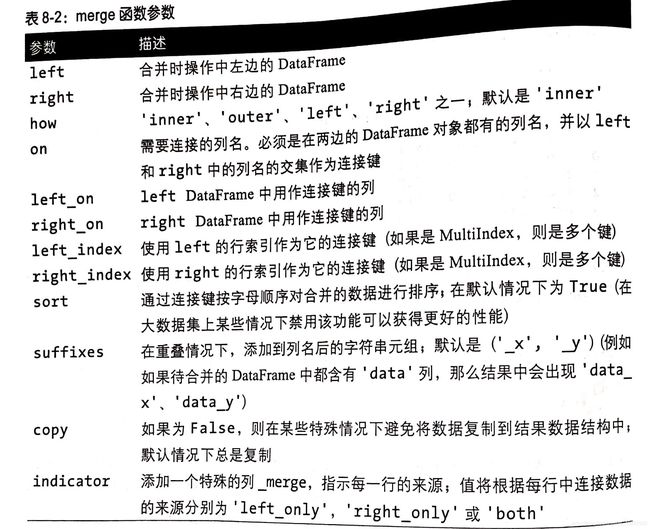
十五、Pandas怎样实现Merge

1、
示例代码：

import pandas as pd

# 设置显示的最大列数
pd.set_option("display.max_columns", 20)
# 读取用户的信息
df_user = pd.read_csv('./ml-1m/users.dat', sep="::", engine="python",
                      names="UserID::Gender::Age::Occupation::Zip-code".split("::"))
# 读取评分的信息
df_rating = pd.read_csv('./ml-1m/ratings.dat', sep="::", engine="python",
                        names="UserID::MovieID::Rating::Timestamp".split("::"))
# 读取电影的信息
df_Movies = pd.read_csv('./ml-1m/movies.dat', sep="::", engine="python",
                        names="MovieID::Title::Genres".split("::"))
# 将用户和评分的合并
df_rating_user = pd.merge(df_rating, df_user, left_on="UserID", right_on="UserID", how="inner")
# 全部合并
df_rating_user_movie = pd.merge(df_rating_user, df_Movies, left_on="MovieID", right_on="MovieID", how="inner")

df_rating_user_movie.to_csv("merge.csv", index=False)

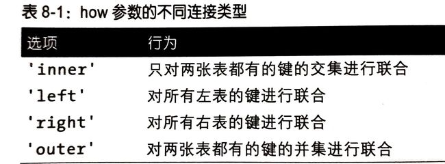
2、理解merge的数量对齐关系

• one-to-one：一对一的关系，关联的key都是唯一的
  • 比如：（学号，姓名）merge（学号，年龄）
  • 结果条数：1*1
    示例代码：

import pandas as pd

'''
one-to-one一对一关系的merge
'''
left = pd.DataFrame({'sno': [11, 12, 13, 14], 'name': ['a', 'b', 'c', 'd']})
right = pd.DataFrame({'sno': [11, 12, 13, 14], 'age': [21, 11, 22, 23]})
l_r = pd.merge(left, right, on='sno')
print(l_r)
输出结果：
   sno name  age
0   11    a   21
1   12    b   11
2   13    c   22
3   14    d   23

• one-to-many：一对多的关系，左边唯一key，右边不唯一key
  • 比如：（学号，姓名）merge（学号，[语文成绩，数学成绩， 英语成绩]）
  • 结果条数：1*N
    示例代码：

import pandas as pd

'''
one-to-many一对多关系的merge
'''
left = pd.DataFrame({'sno': [11, 12, 13, 14], 'name': ['a', 'b', 'c', 'd']})
right = pd.DataFrame({'sno': [11, 11, 11, 12, 12, 13], 'grade': ['语文88', '数学90', '英语75', '语文66', '数学55', '英语29']})
print(left)
输出结果：
   sno name
0   11    a
1   12    b
2   13    c
3   14    d
print(right)
输出结果：
   sno grade
0   11  语文88
1   11  数学90
2   11  英语75
3   12  语文66
4   12  数学55
5   13  英语29
print(pd.merge(left, right, on='sno'))
输出结果：
   sno name grade
0   11    a  语文88
1   11    a  数学90
2   11    a  英语75
3   12    b  语文66
4   12    b  数学55
5   13    c  英语29

• many-to-many：多对多的关系，左边右边都不是唯一的
  • 比如：（学号，[语文成绩，数学成绩， 英语成绩]）merge（学号，[篮球，乒乓球，足球]）
  • 结果条数：M*N
    示例代码：

import pandas as pd

'''
many-to-many多对多的merge
'''
left = pd.DataFrame({'sno': [11, 11, 12, 12, 12], '爱好': ['足球', '篮球', '乒乓球', '羽毛球', '排球']})
right = pd.DataFrame({'sno': [11, 11, 11, 12, 12, 13], 'grade': ['语文88', '数学90', '英语75', '语文66', '数学55', '英语29']})
print(left)
输出结果：
   sno   爱好
0   11   足球
1   11   篮球
2   12  乒乓球
3   12  羽毛球
4   12   排球
print(right)
输出结果：
   sno grade
0   11  语文88
1   11  数学90
2   11  英语75
3   12  语文66
4   12  数学55
5   13  英语29
print(pd.merge(left, right, on='sno'))
输出结果：
    sno   爱好 grade
0    11   足球  语文88
1    11   足球  数学90
2    11   足球  英语75
3    11   篮球  语文88
4    11   篮球  数学90
5    11   篮球  英语75
6    12  乒乓球  语文66
7    12  乒乓球  数学55
8    12  羽毛球  语文66
9    12  羽毛球  数学55
10   12   排球  语文66
11   12   排球  数学55

出现非key的字段重名
示例代码：

import pandas as pd

'''
非key字段重名
'''
left = pd.DataFrame({'key': ['K0', 'K1', 'K2', 'K3'],
                     'A': ['A0', 'A1', 'A2', 'A3'],
                     'B': ['B0', 'B1', 'B2', 'B3']
                     })
right = pd.DataFrame({'key': ['K0', 'K1', 'K4', 'K5'],
                      'A': ['A10', 'A11', 'A12', 'A13'],
                      'D': ['D0', 'D1', 'D2', 'D3']
                      })
print(left)
输出结果：
  key   A   B
0  K0  A0  B0
1  K1  A1  B1
2  K2  A2  B2
3  K3  A3  B3
print(right)
输出结果：
  key    A   D
0  K0  A10  D0
1  K1  A11  D1
2  K4  A12  D2
3  K5  A13  D3
# pandas默认的how=inner
print(pd.merge(left, right, on='key'))
输出结果：
  key A_x   B  A_y   D
0  K0  A0  B0  A10  D0
1  K1  A1  B1  A11  D1
print(pd.merge(left, right, on='key',suffixes=('_left', '_right')))
输出结果：
  key A_left   B A_right   D
0  K0     A0  B0     A10  D0
1  K1     A1  B1     A11  D1

十六、Pandas实现数据的合并concat

• 使用场景：批量合并相同格式的Excel、给DataFrame添加行、给DataFrame添加列
• 一句话说明concat语法“
  • 使用某种合并方式（inner/outer）
  • 沿这某个轴向（axis=0/1）
  • 把多个Pandas对象（DataFrame/Series）合并成一个。
• concat的语法：pandas.concat(objs, axis= 0, join=“outer”, ignore_index=False)
  • objs: 一个列表，内容可以是DataFrame或者Series，可以混合
  • axis：默认是0代表按行合并，如果等于1代表按列合并
  • join：合并的时候索引的对齐方式，默认是outer join， 也可以是inner join
  • ignore_index: 是否忽略掉原来的数据索引

import pandas as pd
import warnings

warnings.filterwarnings('ignore')
df1 = pd.DataFrame({'A': ['A0', 'A1', 'A2', 'A3'],
                    'B': ['B0', 'B1', 'B2', 'B3'],
                    'C': ['C0', 'C1', 'C2', 'C3'],
                    'D': ['D0', 'D1', 'D2', 'D3'],
                    'E': ['E0', 'E1', 'E2', 'E3'],
                    })
df2 = pd.DataFrame({'A': ['A4', 'A5', 'A6', 'A7'],
                    'B': ['B4', 'B5', 'B6', 'B7'],
                    'C': ['C4', 'C5', 'C6', 'C7'],
                    'D': ['D4', 'D5', 'D6', 'D7'],
                    'F': ['F4', 'F5', 'F6', 'F7'],
                    })
# 使用Concat合并,默认为axis=0,join="outer", ignore_index=False
mer1 = pd.concat([df1, df2], join="inner", ignore_index=True)
print(mer1)
输出结果：
    A   B   C   D
0  A0  B0  C0  D0
1  A1  B1  C1  D1
2  A2  B2  C2  D2
3  A3  B3  C3  D3
4  A4  B4  C4  D4
5  A5  B5  C5  D5
6  A6  B6  C6  D6
7  A7  B7  C7  D7
mer2 = pd.concat([df1, df2], axis=1, join="inner", ignore_index=True)
print(mer2)
输出结果：
    0   1   2   3   4   5   6   7   8   9
0  A0  B0  C0  D0  E0  A4  B4  C4  D4  F4
1  A1  B1  C1  D1  E1  A5  B5  C5  D5  F5
2  A2  B2  C2  D2  E2  A6  B6  C6  D6  F6
3  A3  B3  C3  D3  E3  A7  B7  C7  D7  F7

• appen语法：DataFrame.append(other, ignore_index=False)
  append只有按行合并，没有按列合并，相当于concat按行的简写形式
  • other： 单个dataframe、series、dict、或者列表
  • ignore_index: 是否忽略原来的数据索引。

import pandas as pd
import warnings

warnings.filterwarnings('ignore')
# 使用DataFrame.append按行合并数据
df3 = pd.DataFrame([[1, 2], [3, 4]], columns=list('AB'))
df4 = pd.DataFrame([[5, 6], [7, 8]], columns=list('AB'))
# 1、给一个DataFrame添加另一个DataFrame,ignore_index=False为忽略原来的索引
appen = df3.append(df4, ignore_index="True")
print(appen)
输出结果：
   A  B
0  1  2
1  3  4
2  5  6
3  7  8
# 2、一行一行的给DataFrame添加数据
df5 = pd.DataFrame(columns=['A'])
# 低性能版本
for i in range(5):
    # 注意这里每次都在复制
    df5 = df5.append({'A': i}, ignore_index=True)
print(df5)
输出结果：
   A
0  0
1  1
2  2
3  3
4  4
# 性能好的版本，第一个入参的是一个列表，避免了多次复制
df6 = pd.concat([pd.DataFrame([i], columns=['A']) for i in range(5)], ignore_index=True)
print(df6)
输出结果：
   A
0  0
1  1
2  2
3  3
4  4

十七、Pandas批量拆分与合并

1、批量拆分示例代码：

import pandas as pd

pd.set_option('display.max_columns', 10)
df = pd.read_excel('example.xlsx')
# 将大的excel分给以下几个人
user_names = ["xiaohong", "xiaoming", "xiaowang"]
# 获取总的任务数
total_size = df.shape[0]
# 每个人处理的数量
split_size = total_size // len(user_names)
# 判断是否除的尽，如果除不尽则前面的人多处理一份
if total_size % len(user_names) != 0:
    split_size += 1

df_subs = []
# 获取用户名的序号和名字
for idx, user_name in enumerate(user_names):
    # iloc的开始索引
    begin = idx * split_size
    # print(begin)
    # iloc的结束的索引
    end = begin + split_size
    # 实现df按照iloc拆分
    df_sub = df.iloc[begin:end]
    # 将每个子df存入列表
    df_subs.append((idx, user_name, df_sub))
for idx, user_name, df_sub in df_subs:
    file_name = f"{idx}_{user_name}.xlsx"
    df_sub.to_excel(file_name, index=False)

2、批量合并示例代码：

import pandas as pd
import os

# 遍历文件夹，得到要合并的Excel名称列表
excel_names = []
for excel_name in os.listdir("concat_merge"):
    excel_names.append(excel_name)
# 分别读取到DataFrame
df_list = []
for excel_name in excel_names:
    # 读取每个excel到df
    excel_path = f"{'concat_merge'}/{excel_name}"
    df_split = pd.read_excel(excel_path)
    # 获取用户名
    username = excel_name[0:10]
    # 添加一列username
    df_split['username'] = username
    df_list.append(df_split)

# 使用concat合并
df_merge = pd.concat(df_list)
# 保存到excel
df_merge.to_excel("concat_merge_copy.xlsx", index=False)

十八、Pandas怎样实现groupby分组统计

groupby:先对数据进行分组，然后在每个分组上应用聚合函数、转换函数
本次演示：
1、分组使用聚合函数做数据统计
2、遍历groupby的结果理解执行流程
3、实例分组探索天气数据、
示例代码：

import pandas as pd
import numpy as np
from matplotlib.pyplot import plot

df = pd.DataFrame({'A': ['foo', 'bar', 'foo', 'bar', 'foo', 'bar', 'foo', 'foo'],
                   'B': ['one', 'one', 'two', 'three', 'two', 'two', 'one', 'three'],
                   'C': np.random.randn(8),
                   'D': np.random.randn(8)
                   })
print(df)
输出结果：
     A      B         C         D
0  foo    one  0.047047 -0.081082
1  bar    one  0.573521  0.097808
2  foo    two  0.097338  0.527937
3  bar  three  0.909474 -0.079528
4  foo    two -0.459937 -1.211283
5  bar    two -1.226424 -0.415521
6  foo    one  0.012840 -1.547902
7  foo  three -0.987717 -0.982083
# 一、分组使用聚合函数做数据统计
# 1、单个列groupby，查询所有数据列的统计。A列变成了索引，B列不是数字列，自动忽略掉。
print(df.groupby('A').sum())
输出结果：
            C         D
A                      
bar  0.256571 -0.397240
foo -1.290428 -3.294413
# 2、多个列groupby，查询所有数据的统计
print(df.groupby(['A', 'B']).mean())
输出结果：
                  C         D
A   B                        
bar one    0.573521  0.097808
    three  0.909474 -0.079528
    two   -1.226424 -0.415521
foo one    0.029944 -0.814492
    three -0.987717 -0.982083
    two   -0.181299 -0.341673
# as_index=False为不让A，B变成索引值
print(df.groupby(['A', 'B'], as_index=False).mean())
输出结果：
     A      B         C         D
0  bar    one  0.573521  0.097808
1  bar  three  0.909474 -0.079528
2  bar    two -1.226424 -0.415521
3  foo    one  0.029944 -0.814492
4  foo  three -0.987717 -0.982083
5  foo    two -0.181299 -0.341673
# 3、同时查看多种数据统计
#   （1）、预过滤，性能更好
print(df.groupby('A').agg([np.sum, np.mean, np.std]))
输出结果：
            C                             D                    
          sum      mean       std       sum      mean       std
A                                                              
bar  0.256571  0.085524  1.148530 -0.397240 -0.132413  0.260719
foo -1.290428 -0.258086  0.465279 -3.294413 -0.658883  0.857665
          sum      mean       std
# 筛选出C列做数据统计
print(df.groupby('A')['C'].agg([np.sum, np.mean, np.std]))
输出结果：
          sum      mean       std
A                                
bar  0.256571  0.085524  1.148530
foo -1.290428 -0.258086  0.465279
# 不同列使用不同的聚合函数
print(df.groupby('A').agg({"C": np.sum, "D": np.mean}))
输出结果：
            C         D
A                      
bar  0.256571 -0.132413
foo -1.290428 -0.658883
# 二、遍历groupby的结果理解执行流程， for循环可以直接遍历每个group
# 1、遍历单个列聚合的分组
g = df.groupby('A')
for i in g:
    print(i)
 输出结果：
 ('bar',      A      B         C         D
1  bar    one  0.573521  0.097808
3  bar  three  0.909474 -0.079528
5  bar    two -1.226424 -0.415521)
('foo',      A      B         C         D
0  foo    one  0.047047 -0.081082
2  foo    two  0.097338  0.527937
4  foo    two -0.459937 -1.211283
6  foo    one  0.012840 -1.547902
7  foo  three -0.987717 -0.982083)

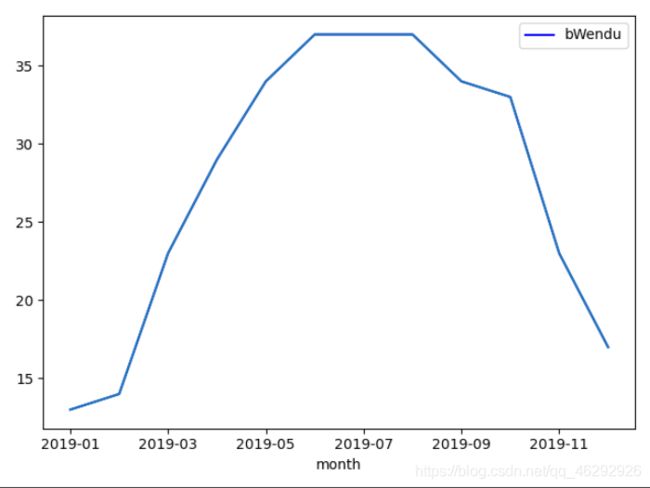
探索天气数据实例演示代码1：

import pandas as pd
import numpy as np
import matplotlib.pyplot as plt

df = pd.read_csv('all_year_weather2019.csv', encoding='gbk')
df.loc[:, "bWendu"] = df["bWendu"].str.replace("℃", "").astype("int32")
df.loc[:, "yWendu"] = df["yWendu"].str.replace("℃", "").astype("int32")

# 新增一列为月份
df['month'] = df['ymd'].str[0:7]
# 绘制月最高温图
hwd = df.groupby('month')['bWendu'].max()[::1]
# 设置颜色及标签
hwd.plot(color='blue', legend=True)
# 绘图
plt.plot(hwd)
plt.show()

输出结果：

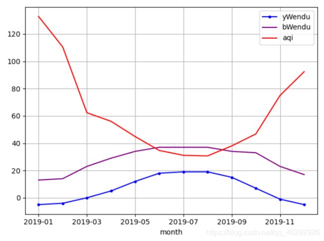
探索天气数据实例演示代码2：

import pandas as pd
import numpy as np
import matplotlib.pyplot as plt

df = pd.read_csv('all_year_weather2019.csv', encoding='gbk')
df.loc[:, "bWendu"] = df["bWendu"].str.replace("℃", "").astype("int32")
df.loc[:, "yWendu"] = df["yWendu"].str.replace("℃", "").astype("int32")

# 新增一列为月份
df['month'] = df['ymd'].str[0:7]
# 查看月的最高温度，最低温度，平均空气质量指数
many_data = df.groupby('month').agg({'bWendu': np.max, 'yWendu': np.min, 'aqi': np.mean})[::1]
# 最高温
df_hw = many_data['bWendu']
# 最低温
df_lw = many_data['yWendu']
# 平均空气质量指数
df_aqi = many_data['aqi']
# 添加标签,color指定颜色，style指定线条样式
df_lw.plot(color='blue',style=".-", legend=True)
df_hw.plot(color='purple', legend=True)
df_aqi.plot(color='red', legend=True)
# 绘制网格
plt.grid()
# 绘制图像
plt.show()

输出结果：

十九、Pandas的分层索引Multilndex

为什么要学习分层索引Multilndex？

• 分层索引：在一个轴向上拥有多个索引层级，可以表达更高维度数据的形式。
• 可以更方便的进行数据的筛选，如果有序，效果更好
• groupby等的操作结果，如果是多key，结果是分层索引，需要用到
• 一般不需要自己创建分层索引的（Multilndex有构造函数但一般不用）
  示例代码：

import pandas as pd

# 设置显示的最大的列数
pd.set_option('display.max_columns', 11)
# 读取文件
df = pd.read_excel('stock.xlsx')
print(df.head(3))
输出结果：
  trade_date ts_code   open   high    low  close  pre_close  change  pct_chg  \
0    20200911    GNKJ  22.55  23.08  22.23  22.99      22.53    0.46   2.0417   
1    20200910    GNKJ  23.40  23.53  22.28  22.53      23.32   -0.79  -3.3877   
2    20200909    GNKJ  23.46  23.68  23.04  23.32      23.96   -0.64  -2.6711   

        vol     amount  
0  13698.88  31234.914  
1  19295.37  44258.296  
2  18350.09  42877.476  
# 打印三个公司收盘价的平均值
print(df.groupby('ts_code')['close'].mean())
输出结果：
ts_code
GNKJ      22.946667
PAYH    1708.933333
WKA       28.146667
Name: close, dtype: float64
'''
一、Series的分层索引MultiIndex
'''
# 多维索引中，空白的意思是：使用上面的值
# 多key聚合
ser = df.groupby(['ts_code', 'trade_date'])['close'].mean()
print(ser)
输出结果：
ts_code  trade_date
GNKJ     20200909        23.32
         20200910        22.53
         20200911        22.99
PAYH     20200909      1688.00
         20200910      1705.80
         20200911      1733.00
WKA      20200909        27.98
         20200910        28.46
         20200911        28.00
Name: close, dtype: float64
# unstack把二级索引变成列
print(ser.unstack())
输出结果：
trade_date  20200909  20200910  20200911
ts_code                                 
GNKJ           23.32     22.53     22.99
PAYH         1688.00   1705.80   1733.00
WKA            27.98     28.46     28.00
# 把索引变为列
print(ser.reset_index())
输出结果：
  ts_code  trade_date    close
0    GNKJ    20200909    23.32
1    GNKJ    20200910    22.53
2    GNKJ    20200911    22.99
3    PAYH    20200909  1688.00
4    PAYH    20200910  1705.80
5    PAYH    20200911  1733.00
6     WKA    20200909    27.98
7     WKA    20200910    28.46
8     WKA    20200911    28.00
'''
二、Series有多层索引MultiIndex怎么筛选数据
'''
# 单个索引
print(ser.loc['GNKJ'])
输出结果：
trade_date
20200909    23.32
20200910    22.53
20200911    22.99
Name: close, dtype: float64
# 多次索引，可以使用元组的形式筛选
print(ser.loc[('GNKJ', 20200910)])
输出结果：
22.53
# :表示第一级索引全选,第二级索引选择20200909
print(ser.loc[:, 20200909])
输出结果：
ts_code
GNKJ      23.32
PAYH    1688.00
WKA       27.98
Name: close, dtype: float64
'''
DataFrame有多层索引MultiIndex怎么筛选数据：
在选择数据时，
元组(key1, key2)代表筛选多层索引，其中key1时索引第一级，比如key1=GNKJ，key2=20200909
列表[key1, key2]代表同一层的多个key，其中key1和key2是并列的同级索引，比如key1=GNKJ，key2=PAYH
'''
# 设置多层索引
ret = df.set_index(['ts_code', 'trade_date'])
# 进行排序
print(df.sort_index)
输出结果：
<bound method DataFrame.sort_index of    trade_date ts_code     open     high      low    close  pre_close  change  \
0    20200911    GNKJ    22.55    23.08    22.23    22.99      22.53    0.46   
1    20200910    GNKJ    23.40    23.53    22.28    22.53      23.32   -0.79   
2    20200909    GNKJ    23.46    23.68    23.04    23.32      23.96   -0.64   
3    20200911    PAYH  1688.00  1736.00  1688.00  1733.00    1705.80   27.20   
4    20200910    PAYH  1703.74  1720.00  1700.00  1705.80    1688.00   17.80   
5    20200909    PAYH  1699.67  1711.00  1680.04  1688.00    1711.40  -23.40   
6    20200911     WKA    28.46    28.46    27.90    28.00      28.46   -0.46   
7    20200910     WKA    28.36    29.10    28.36    28.46      27.98    0.48   
8    20200909     WKA    28.10    28.40    27.65    27.98      28.30   -0.32   

   pct_chg        vol       amount  
0   2.0417   13698.88    31234.914  
1  -3.3877   19295.37    44258.296  
2  -2.6711   18350.09    42877.476  
3   1.5946   31088.00  5339883.408  
4   1.0545   24778.33  4236694.402  
5  -1.3673   25963.55  4401806.095  
6  -1.6163  541108.37  1519932.745  
7   1.7155  954676.62  2741079.761  
8  -1.1307  645614.25  1807367.850  >
'''
DataFrame有多层索引怎么筛选数据
'''
# 筛选GNKJ的数据
print(ret.loc['GNKJ'])
输出结果：
             open   high    low  close  pre_close  change  pct_chg       vol  \
trade_date                                                                     
20200911    22.55  23.08  22.23  22.99      22.53    0.46   2.0417  13698.88   
20200910    23.40  23.53  22.28  22.53      23.32   -0.79  -3.3877  19295.37   
20200909    23.46  23.68  23.04  23.32      23.96   -0.64  -2.6711  18350.09   

               amount  
trade_date             
20200911    31234.914  
20200910    44258.296  
20200909    42877.476
# 同时实现多层索引,返回当天的全部数据
print(ret.loc[('GNKJ', 20200909), :])
输出结果：
open            23.4600
high            23.6800
low             23.0400
close           23.3200
pre_close       23.9600
change          -0.6400
pct_chg         -2.6711
vol          18350.0900
amount       42877.4760
Name: (GNKJ, 20200909), dtype: float64
# 列表索引
print(ret.loc[['GNKJ', 'WKA'], :])
输出结果：
                     open   high    low  close  pre_close  change  pct_chg  \
ts_code trade_date                                                           
GNKJ    20200911    22.55  23.08  22.23  22.99      22.53    0.46   2.0417   
        20200910    23.40  23.53  22.28  22.53      23.32   -0.79  -3.3877   
        20200909    23.46  23.68  23.04  23.32      23.96   -0.64  -2.6711   
WKA     20200911    28.46  28.46  27.90  28.00      28.46   -0.46  -1.6163   
        20200910    28.36  29.10  28.36  28.46      27.98    0.48   1.7155   
        20200909    28.10  28.40  27.65  27.98      28.30   -0.32  -1.1307   

                          vol       amount  
ts_code trade_date                          
GNKJ    20200911     13698.88    31234.914  
        20200910     19295.37    44258.296  
        20200909     18350.09    42877.476  
WKA     20200911    541108.37  1519932.745  
        20200910    954676.62  2741079.761  
        20200909    645614.25  1807367.850  
# 混合筛选
print(ret.loc[(['GNKJ', 'WKA'], 20200909), 'close'])
输出结果：
ts_code  trade_date
GNKJ     20200909      23.32
WKA      20200909      27.98
Name: close, dtype: float64
print(ret.loc[('WKA', [20200909, 20200911]), 'close'])
输出结果：
ts_code  trade_date
WKA      20200911      28.00
         20200909      27.98
Name: close, dtype: float64
# slice(None)代表筛选索引的所有内容
print(ret.loc[(slice(None), [20200909, 20200911]), :])
输出结果：
                       open     high      low    close  pre_close  change  \
ts_code trade_date                                                          
GNKJ    20200911      22.55    23.08    22.23    22.99      22.53    0.46   
        20200909      23.46    23.68    23.04    23.32      23.96   -0.64   
PAYH    20200911    1688.00  1736.00  1688.00  1733.00    1705.80   27.20   
        20200909    1699.67  1711.00  1680.04  1688.00    1711.40  -23.40   
WKA     20200911      28.46    28.46    27.90    28.00      28.46   -0.46   
        20200909      28.10    28.40    27.65    27.98      28.30   -0.32   

                    pct_chg        vol       amount  
ts_code trade_date                                   
GNKJ    20200911     2.0417   13698.88    31234.914  
        20200909    -2.6711   18350.09    42877.476  
PAYH    20200911     1.5946   31088.00  5339883.408  
        20200909    -1.3673   25963.55  4401806.095  
WKA     20200911    -1.6163  541108.37  1519932.745  
        20200909    -1.1307  645614.25  1807367.850  

二十、Pandas的map-apply-applymap数据转换

map：只能用于Series，实现每个值到值的映射
apply：用于Series实现每个值的处理，用于DataFrame实现某个轴的Series的处理
applymap：只能用于DataFrame，用于处理该DataFrame的每个元素
示例代码：

import pandas as pd

pd.set_option('display.max_columns', 11)
# map：只能用于Series，实现每个值到值的映射
# apply：用于Series实现每个值的处理，用于DataFrame实现某个轴的Series的处理
# applymap：只能用于DataFrame，用于处理该DataFrame的每个元素

'''
一、map用于Series值的转换
Series.map(dict)或者Series.map(function)
'''
# 示例：将股票代码转换为中文名字。
df = pd.read_excel('stock.xlsx')
# print(df.head())
dict_company_name = {
    'GNKJ': '国民科技',
    'PAYH': '平安银行',
    'WKA': '万科A'
}
# 方法1：Series.map(dict)
df['cha1'] = df['ts_code'].map(dict_company_name)
print(df)
# 方法2：Series.map(function)
df['cha2'] = df['ts_code'].map(lambda x: dict_company_name[x])
print(df)
'''
二、apply用于Series和DataFrame的转换
Series.apply(function)函数的参数是每个值
DataFrame.apply(function)函数的参数是Series
'''
# Series.apply(function)，function的参数是Series的每个值
df['cha3'] = df['ts_code'].apply(lambda x: dict_company_name[x])
print(df)
# DataFrame.apply(function)，function的参数是对应轴的Series
df['cha4'] = df.apply(lambda x: dict_company_name[x['ts_code']], axis=1)
print(df)
'''
三、DataFrame使用applymap修改所有的值
'''
sub_df = df[['open', 'high', 'low', 'close', 'pre_close']]
df.loc[:, ['open', 'high', 'low', 'close', 'pre_close']] = sub_df.applymap(lambda x: int(x))
print(df)

二十一、Pandas实现groupby每个分组的apply

GroupBy.apply(function)

• function的第一个参数是DataFrame
• function的返回结果，可以是DataFrame、Series、单个值、甚至和输入的DATa Frame完全没关系。
  实例演示：
  1、怎样对数值按列分组归一化
  2、怎样取每个分组的TOPN数据
  实例一：怎样对数值列按分组的归一化
  将不同范围的数值按列进行归一化，映射到[0, 1]区间上。
• 更容易做数据横向对比，比如价格字段是几百到几千，增幅字段是0到100
• 机器学习模型学的更快性能更好
  用户对电影评分归一化实例代码：

import pandas as pd

'''
实例1：用户对电影评分归一化
'''
ratings = pd.read_csv('./ml-1m/ratings.dat', sep='::', engine='python',
                      names="UserID::MovieID::Rating::Timestamp".split("::"))


def ratings_norm(df):
    """
    @param df:每个用户分组的DataFrame
    """
    min_value = df['Rating'].min()
    max_value = df['Rating'].max()
    df['Rating_norm'] = df['Rating'].apply(lambda x: ((x - min_value) / (max_value - min_value)))
    return df


ratings = ratings.groupby("UserID").apply(ratings_norm)
ret = ratings[ratings["UserID"] == 1]
print(ret.head())

怎样取每个分组的TOPN数据？

import pandas as pd

'''
实例2：怎样取每个分组的TOPN数据？
'''
df = pd.read_csv('weather.csv', encoding='Gbk')
df.loc[:, 'bWendu'] = df['bWendu'].str.replace('℃', '').astype('int32')
df.loc[:, 'yWendu'] = df['yWendu'].str.replace('℃', '').astype('int32')
df['month'] = df['ymd'].str[0:6]


def getWenduTOPN(df, top):
    return df.sort_values(by="bWendu")[['ymd', 'bWendu']][-top:]


print(df.groupby('month').apply(getWenduTOPN, 3))

二十二、pandas使用stock和pivot实现数据透视

将列式数据变成交叉形式，便于分析，叫做重塑或透视
1、经过统计得到多维度指标数据
2、使用unstack实现数据维透视
3、使用pivot简化透视
4、stack、unstack、pivot的语法
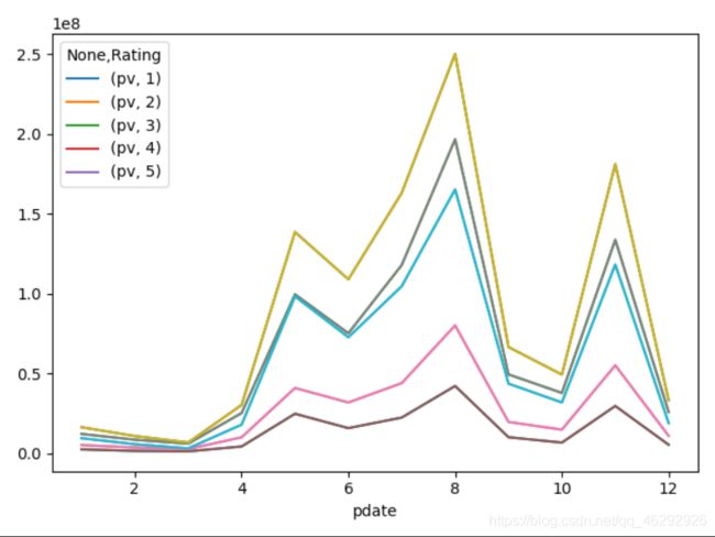
一、使用unstack实现数据二维透视示例代码：

import pandas as pd
import numpy as np
import matplotlib.pyplot as plt

# 将列式数据变成交叉形式，便于分析，叫做重塑或透视
df = pd.read_csv('./ml-1m/ratings.dat', sep='::', engine='python',
                 names="UserID::MovieID::Rating::Timestamp".split("::"))
# 添加一列，将时间戳转换为日期形式。
df['pdate'] = pd.to_datetime(df['Timestamp'], unit='s')
#
df_group = df.groupby([df["pdate"].dt.month, "Rating"])['UserID'].agg(pv=np.sum)
# 使用unstack实现数据二维透视。目的：想要画图对比按照月份的不同评分的数量趋势。
df_unstack = df_group.unstack()
df_unstack.plot()
plt.plot(df_unstack)
plt.show()

输出结果：

• unstack和stack是互逆操作。
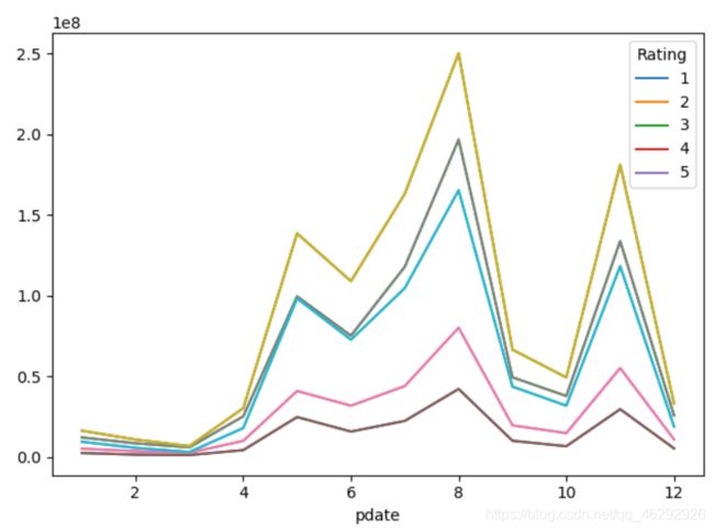
  二、使用pivot简化透视
  pivot方法相当于对df使用set_index创建分层索引，然后调用unstack
  示例代码：

import pandas as pd
import numpy as np
import matplotlib.pyplot as plt

# 将列式数据变成交叉形式，便于分析，叫做重塑或透视
df = pd.read_csv('./ml-1m/ratings.dat', sep='::', engine='python',
                 names="UserID::MovieID::Rating::Timestamp".split("::"))
# 添加一列，将时间戳转换为日期形式。
df['pdate'] = pd.to_datetime(df['Timestamp'], unit='s')
#
df_group = df.groupby([df["pdate"].dt.month, "Rating"])['UserID'].agg(pv=np.sum)
# 重新设置索引
df_reset = df_group.reset_index()
# pivot参数分别代表x，y，值。
df_pivot = df_reset.pivot('pdate', 'Rating', 'pv')
df_pivot.plot()
plt.plot(df_pivot)
plt.show()

输出结果：

二十三、Pandas快速实现周，月，季度的日期聚合统计

Pandas日期处理的作用：将多种日期格式转换成统一的格式对象，在该对象上提供强大的功能支持。
几个概念：
1、pd.to_datetime：Pandas的一个函数，能将字符串、列表、Series变成日期格式
2、TimeStamp：Pandas表示日期的对象形式
3、DatatimeIndex：Pandas表示日期的对象列表形式
其中：

• DatetimeIndex是TimeStamp的列表形式
• pd.to_datetime对单个日期字符处理得到TimeStamp
• pd.to_datetime对日期字符串处理会得到Datetimeindex
  示例代码：

import pandas as pd
import matplotlib.pyplot as plt

# 读取数据
df = pd.read_csv('all_year_weather2019.csv', encoding='gbk')
df.loc[:, 'bWendu'] = df['bWendu'].str.replace('℃', '').astype('int32')
df.loc[:, 'yWendu'] = df['yWendu'].str.replace('℃', '').astype('int32')
# 将日期转换成pandas的日期,并转换为索引列
ret = df.set_index(pd.to_datetime(df['ymd']))
# 筛选某一天的数据
day = ret.loc["2019-03-02"]
print(day)
# 筛选日期去区间的数据,中间为冒号分隔
day_gap = ret.loc['2019-03':'2019-06']
print(day_gap)
# 按年份查询
year = ret.loc['2019']
print(year)

获取周、月、季度信息示例代码：

import pandas as pd
import matplotlib.pyplot as plt

# 读取数据
df = pd.read_csv('all_year_weather2019.csv', encoding='gbk')
df.loc[:, 'bWendu'] = df['bWendu'].str.replace('℃', '').astype('int32')
df.loc[:, 'yWendu'] = df['yWendu'].str.replace('℃', '').astype('int32')
# 将日期转换成pandas的日期,并转换为索引列
ret = df.set_index(pd.to_datetime(df['ymd']))
'''
获取周、月、季度信息
'''
# 获取周数字列
week = ret.index.week
print(week)
# 获取周数字列
month = ret.index.month
print(month)
quarter = ret.index.quarter
print(quarter)

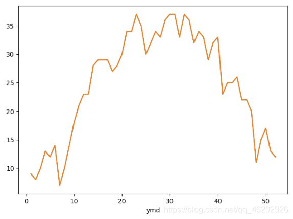
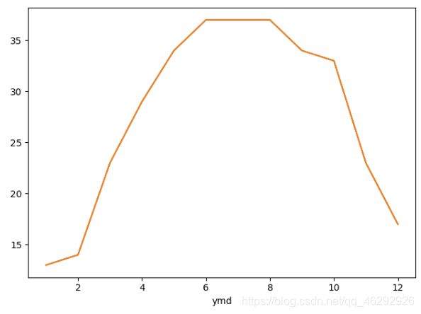
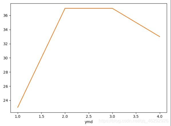
统计周、月、季度的最高温度示例代码：

import pandas as pd
import matplotlib.pyplot as plt

# 读取数据
df = pd.read_csv('all_year_weather2019.csv', encoding='gbk')
df.loc[:, 'bWendu'] = df['bWendu'].str.replace('℃', '').astype('int32')
df.loc[:, 'yWendu'] = df['yWendu'].str.replace('℃', '').astype('int32')
# 将日期转换成pandas的日期,并转换为索引列
ret = df.set_index(pd.to_datetime(df['ymd']))
'''
统计周、月、季度的最高温度
'''
# 统计周最高温度
week_bWendu = ret.groupby(ret.index.week)['bWendu'].max()
week_bWendu.plot()
plt.plot(week_bWendu)
plt.show()
# 统计月最高温度
month_bWendu = ret.groupby(ret.index.month)['bWendu'].max()
month_bWendu.plot()
plt.plot(month_bWendu)
plt.show()
# 统计季度最高温度
quarter_bWendu = ret.groupby(ret.index.quarter)['bWendu'].max()
quarter_bWendu.plot()
plt.plot(quarter_bWendu)
plt.show()

输出结果：

二十四、Pandas处理日期索引的缺失

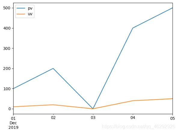
使用reindex方法示例代码：

import pandas as pd
import matplotlib.pyplot as plt

# 创建DaraFrane对象，缺少2019-12-03的日期
df = pd.DataFrame({
    "pdate": ["2019-12-01", "2019-12-02", "2019-12-04", "2019-12-05"],
    "pv": [100, 200, 400, 500],
    "uv": [10, 20, 40, 50]
})
# 将df的索引列变成日期索引
ret = df.set_index('pdate')
# 将日期索引类型变成datetime类型
df_ret = ret.set_index(pd.to_datetime(ret.index))
'''
方法1：使用Pandas的reindex方法
'''
# 生成完整的日期序列
date_range = pd.date_range(start='2019-12-01', end='2019-12-05')
# reindex方法，fill_value为空缺日期的填充值
new_date = df_ret.reindex(date_range, fill_value=0)
# 绘图
new_date.plot()
plt.plot(new_date )
plt.show()

输出结果：

resample的含义：改变数据的时间频率，比如把天数据变成月份，或者把小时数据变成分钟级别
语法：（DataFrame or Series）.resample(arduments).(aggregate function)

使用resample方法示例代码：

import pandas as pd
import matplotlib.pyplot as plt

# 创建DaraFrane对象，缺少2019-12-03的日期
df = pd.DataFrame({
    "pdate": ["2019-12-01", "2019-12-02", "2019-12-04", "2019-12-05"],
    "pv": [100, 200, 400, 500],
    "uv": [10, 20, 40, 50]
})
'''
方法2：使用pandas的resample方法
'''
# drop方法删除保留的pdate的一列，axis=1按列删除
df_resample = df.set_index(pd.to_datetime(df['pdate'])).drop('pdate', axis=1)
# 使用dataframe的resample的方法按照天重采样
'''
resample的含义：改变数据的时间频率，比如把天数据变成月份，或者把小时数据变成分钟级别
语法：（DataFrame or Series）.resample(arduments).(aggregate function)
'''
# 由于采样会让区间变成一个值，所以需要指定mean等采样值的设定方法
# D表示按天采样，M表示按月采样，2D表示按两天采样
new_data1 = df_resample.resample('D').mean().fillna(0)
new_data1.plot()
plt.plot(new_data1)
plt.show()

输出结果：

二十五、Pandas实现Excel的vlookup在指定列后面输出

背景：
1、有两个excel，他们有相同的一列
2、按照这个列合并成一个大的excel，即vlookup功能，要求：

• 只需要第二个excel的少量的列，比如从40个列中挑选2列
• 新增的来自第二个excel的列需要放到第一个excel指定的列后面
  3、将结果输出到一个新的excel

import pandas as pd

'''
1、读取两个文件
'''
# 读取学生成绩表
df_grade = pd.read_excel('StudentsSroce.xlsx')
# 读取学生信息表
df_data = pd.read_excel('StudentsData.xlsx')
'''
2、实现两个表的关联，即excel的vlookup功能
'''
# 只筛选出第二表少量的列
df_data = df_data[['学号', '姓名', '性别']]
# 使用merge实现数据的关联
df_merge = pd.merge(left=df_grade, right=df_data, left_on='学号', right_on='学号')
'''
3、调整列的顺序
'''
# 使用python的语法实现列表的处理
# 将columns变成python列表的形式
new_columns = df_merge.columns.to_list()
# 按逆序insert，会将“姓名”，“性别”放到的学号的后面
for name in ["姓名", "性别"][::-1]:
    new_columns.remove(name)
    new_columns.insert(new_columns.index("学号")+1, name)
    df_merge = df_merge.reindex(columns=new_columns)
# 保存到excel
df_merge.to_excel('Students.xlsx', index=False)

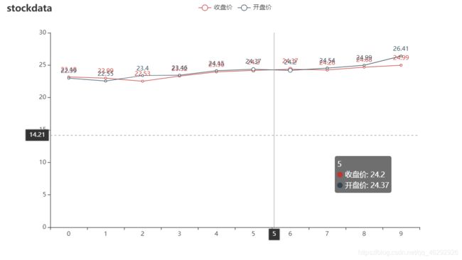
二十六、Pandas读取Excel并绘制图像

import pandas as pd
import tushare as ts
from pyecharts.charts import Line
from pyecharts import options as opts

# tushare的token
token = '5111b5dcfed22c77117bdb338038ded38d75f346c0333423eca884bc'
# 初始化token
pro = ts.pro_api(token)
# 设置显示的最大列数
pd.set_option('display.max_columns', 11)
# 获取日线行情，并转化为DataFrame对象
df = pd.DataFrame(pro.daily(ts_code='000004.SZ', start_date="20200901", end_date='20200914'))
# 取出两列
df_range = df[['trade_date', 'close']]
# 设置索引
df_range.set_index('trade_date')
# 初始化线图
line = Line()
# 添加x轴
line.add_xaxis(df_range.index.to_list())
# 添加y轴
line.add_yaxis("收盘价", df_range['close'].to_list())
# 设置图像
line.set_global_opts(title_opts=opts.TitleOpts(title="估票数据"),
                     tooltip_opts=opts.TooltipOpts(trigger='axis', axis_pointer_type="cross")
                     )
# 加载图像
line.render('stock.html')

输出结果：

二十七、Pandas结合Sklearn实现机器学习

二十八、Pandas实现原始网站日志处理与分析

二十九、Pandas查询数据的简便方法

怎么进行复杂组合条件对数据的查询：

• 方式一、使用(df[df[“a”] > 3]) & (df[df[“b”] < 5)]的方式
• 方式二、使用df.query(“a > 3” & “b < 5”)的方式
  方法二的语法更加简洁
  性能对比：
• 当数据小时，方法一更快
• 当数据大时，因为方法二之直接用C语言实现，节省方法一临时数组的多次复制，方法二更快
  **使用df.query简化查询
  形式：DataFrame.query(expr, inplace=False, kwargs)
  其中expr为要返回boolean结果的字符串表达式
  形如：
  df.query(“a < 100”)
  df.query(‘a < b & b < c’), 或者df.query((a < b) & (b < c))
  df.query可支持的表达式语法：
  逻辑操作符，比较操作符，单变量操作符，多变量操作符
  df.query中可以使用@var的方式传入外部变量
  示例代码：

import pandas as pd

# 读取数据
df = pd.read_csv('all_year_weather2019.csv', encoding='gbk')
df.loc[:, 'bWendu'] = df['bWendu'].str.replace("℃", "").astype('int32')
df.loc[:, 'yWendu'] = df['yWendu'].str.replace("℃", "").astype('int32')
print(df.head())
# 使用PandasFrame条件表达式查询，查询最低温度低于10摄氏度的列表
low_5 = df[df["yWendu"] <= -5]
print(low_5)
# 复杂条件查询。查询最高温度小于30度，并且最低温度大于15度，并且是晴天，并且天气为优的数据
complex_ = df[(df["bWendu"] < 30) & (df["yWendu"] > 15) & (df["tianqi"] == "晴") & (df["aqiLevel"] == 1)]
print(complex_)
'''
使用df.query简化查询
形式：DataFrame.query(expr, inplace=False, **kwargs)
其中expr为要返回boolean结果的字符串表达式
形如：
df.query("a < 100")
df.query('a < b & b < c'), 或者df.query((a < b) & (b < c))
df.query可支持的表达式语法：
逻辑操作符，比较操作符，单变量操作符，多变量操作符
df.query中可以使用@var的方式传入外部变量
'''
# 简单查询
low_query = df.query("yWendu < 3").head()
print(low_query)
# 复杂查询，查询最高温度小于30度，并且最低温度大于15度，并且是晴天，并且天气为优的数据
complex_query = df.query("bWendu < 30 & yWendu > 15 & tianqi == '晴'  & aqiLevel == 1")
print(complex_query)
# 查询温差大于15度的日子
wencha = df.query("bWendu-yWendu > 15")
print(wencha)
# 可以外部变量。查询温度在这两个温度之间的数据
high_temperature = 15
low_temperature = 13
out_wencha = df.query("yWendu <= @high_temperature & yWendu >= @low_temperature")
print(out_wencha)

三十、Pandas按行遍历DataFrame的3种方法

1、df.iterrows方法
示例代码：

import pandas as pd
import numpy as np

df = pd.DataFrame(np.random.random(size=(1000000, 4)), columns=list('ABCD'))
# print(df.head())
# 1、df.iterrows方法
for idx, row in df.iterrows():
    print(idx, row)
    print(idx, row['A'], row['B'], row['C'], row['D'])

2、df.itertuples()
示例代码：

import pandas as pd
import numpy as np

df = pd.DataFrame(np.random.random(size=(1000000, 4)), columns=list('ABCD'))
for row in df.itertuples():
    print(row)
    print(row.Index, row.A, row.B, row.C, row.D)
    break

3、for+zip
既不需要类型检查，也不需要构建namedtuple，缺点是需要指定变量

import pandas as pd
import numpy as np

df = pd.DataFrame(np.random.random(size=(1000000, 4)), columns=list('ABCD'))
for A, B in zip(df['A'], df['B']):
    print(A, B)
    break