读书笔记《Deep Learning for Computer Vision with Python》- 第二卷 第10章 GoogLeNet

下载地址

链接：https://pan.baidu.com/s/1hqtBQf6jRJINx4AgB8S2Tw 
提取码：zxkt 

        第二卷 第十章 GoogLeNet

        在本章中，我们将研究GoogLeNet 架构。 首先，与 AlexNet 和 VGGNet 相比，模型架构很小（权重本身为约28MB）。作者能够通过移除完全连接的层并使用全局平均池化来实现网络架构大小的显着下降（同时仍然增加整个网络的深度）。CNN 中的大部分权重都可以在密集的 FC 层中找到，如果这些层可以被移除，内存节省是巨大的。

        具体来说， Inception 模块是一个适合卷积神经网络的构建块，使其能够学习具有多种过滤器尺寸的 CONV 层，从而将该模块转变为多级特征提取器。

        Inception 等微架构启发了其他重要的变体，包括 ResNet中的 Residual 模块和 SqueezeNet 中的 Fire 模块。我们将在本章后面讨论 Inception 模块（及其变体）。 并了解它的原理，我们将实现一个较小版本的 GoogLeNet，称为“MiniGoogLeNet”——我们将在 CIFAR-10 数据集上训练这个架构，并获得比之前章节任何其他架构更高的准确率。

        之后，我们将继续进行更困难的Tiny ImageNet挑战。这项挑战是为参加斯坦福大学 cs231n 卷积神经网络视觉识别课程的学生提供的。这意味着让体验与现代架构上的大规模深度学习相关的挑战，而不是像整个 ImageNet 数据集那样耗时或费力。

        通过在 Tiny ImageNet 上从头开始训练 GoogLeNet，我们将演示如何在 Tiny ImageNet 排行榜上获得最高排名。 在我们的下一章中，我们将利用 ResNet 从从头开始训练。

        1、Inception 模块（及其变体）

        Inception 模块背后的总体思路有两个方面：

        （1）很难决定在给定的 CONV 层上需要学习的过滤器的大小。5×5还是3×3？或者1×1的过滤器来学习局部特征吗？ 相反，为什么不全部学习它们并让模型决定呢？在 Inception 模块中，我们学习了所有三个 5×5、3×3 和 1×1 过滤器（并行计算它们）沿着通道维度连接生成的特征图。GoogLeNet 架构中的下一层（可能是另一个 Inception 模块）接收这些串联的混合过滤器并执行相同的过程。总的来说，这个过程使 GoogLeNet 能够通过较小的卷积学习局部特征和具有较大卷积的抽象特征——我们不必以牺牲较小的特征为代价来牺牲我们的抽象水平。

        （2）通过学习多个filter-size，我们可以把这个模块变成一个多级特征提取器。5×5个filters有更大的receptive size，可以学习更多的抽象特征。 1×1 过滤器根据定义是本地的。 3×3 过滤器作为两者之间的平衡。

        1.1 Inception

        现在我们已经讨论了 Inception 模块背后的动机，让我们看看图中的实际模块本身。

GoogLeNet 中使用的原始 Inception 模块。 Inception 模块通过在网络的同一模块内计算 1×1、3×3 和 5×5 卷积来充当“多级特征提取器”。

         在每个 CONV 层之后隐式应用激活函数 (ReLU)。 为了节省篇幅，网络图中没有包含这个激活函数。 当我们实现 GoogLeNet 时，您将看到如何在 Inception 模块中使用此激活。

        1.2 Miniception

        最初的 Inception 模块是为 GoogLeNet 设计的，因此它可以在 ImageNet 数据集上进行训练（假设每个输入图像为 224×224×3）并获得最先进的精度。 对于需要较少网络参数的较小数据集（具有较小的图像空间维度），我们可以简化 Inception 模块。

Miniception 架构由构建块组成，包括卷积模块、Inception 模块和 Downsample 模块。

         ·左：负责执行卷积、批量归一化和激活的卷积模块。

        ·中间：Miniception 模块执行两组卷积，一组用于 1×1 过滤器，另一组用于 3×3 过滤器，然后连接结果。 在 3×3 过滤器之前不执行降维，因为 (1) 输入量已经较小（因为我们将使用 CIFAR-10 数据集）和 (2) 以减少网络中的参数数量。

        ·右图：一个下采样模块，它应用卷积和最大池化来降低维度，然后跨过滤器维度连接。

        2、MiniGoogLeNet在CIFAR-10上

        在本节中，我们将使用 Miniception 模块实现 MiniGoogLeNet 架构。 然后我们将在 CIFAR-10 数据集上训练 MiniGoogLeNet。 正如我们的结果将证明的那样，该架构将在 CIFAR-10 上获得 > 90% 的准确率，远好于我们之前的所有尝试。

        2.1 实施MiniGoogLeNet

        创建minigooglenet.py

# import the necessary packages
from tensorflow.keras.layers import BatchNormalization
from tensorflow.keras.layers import Conv2D
from tensorflow.keras.layers import AveragePooling2D
from tensorflow.keras.layers import MaxPooling2D
from tensorflow.keras.layers import Activation
from tensorflow.keras.layers import Dropout
from tensorflow.keras.layers import Dense
from tensorflow.keras.layers import Flatten
from tensorflow.keras.layers import Input
from tensorflow.keras.models import Model
from tensorflow.keras.layers import concatenate
from tensorflow.keras import backend as K

class MiniGoogLeNet:
    @staticmethod
    def conv_module(x, K, kX, kY, stride, chanDim, padding="same"):
        # define a CONV => BN => RELU pattern
        x = Conv2D(K, (kX, kY), strides=stride, padding=padding)(x)
        x = BatchNormalization(axis=chanDim)(x)
        x = Activation("relu")(x)
        # return the block
        return x

    @staticmethod
    def inception_module(x, numK1x1, numK3x3, chanDim):
        # define two CONV modules, then concatenate across the
        # channel dimension
        conv_1x1 = MiniGoogLeNet.conv_module(x, numK1x1, 1, 1, (1, 1), chanDim)
        conv_3x3 = MiniGoogLeNet.conv_module(x, numK3x3, 3, 3, (1, 1), chanDim)
        x = concatenate([conv_1x1, conv_3x3], axis=chanDim)
        # return the block
        return x

    @staticmethod
    def downsample_module(x, K, chanDim):
        # define the CONV module and POOL, then concatenate
        # across the channel dimensions
        conv_3x3 = MiniGoogLeNet.conv_module(x, K, 3, 3, (2, 2), chanDim, padding="valid")
        pool = MaxPooling2D((3, 3), strides=(2, 2))(x)
        x = concatenate([conv_3x3, pool], axis=chanDim)
        # return the block
        return x

    @staticmethod
    def build(width, height, depth, classes):
        # initialize the input shape to be "channels last" and the
        # channels dimension itself
        inputShape = (height, width, depth)
        chanDim = -1

        # if we are using "channels first", update the input shape
        # and channels dimension
        if K.image_data_format() == "channels_first":
            inputShape = (depth, height, width)
            chanDim = 1
        # define the model input and first CONV module
        inputs = Input(shape=inputShape)
        x = MiniGoogLeNet.conv_module(inputs, 96, 3, 3, (1, 1), chanDim)
        # two Inception modules followed by a downsample module
        x = MiniGoogLeNet.inception_module(x, 32, 32, chanDim)
        x = MiniGoogLeNet.inception_module(x, 32, 48, chanDim)
        x = MiniGoogLeNet.downsample_module(x, 80, chanDim)

        # four Inception modules followed by a downsample module
        x = MiniGoogLeNet.inception_module(x, 112, 48, chanDim)
        x = MiniGoogLeNet.inception_module(x, 96, 64, chanDim)
        x = MiniGoogLeNet.inception_module(x, 80, 80, chanDim)
        x = MiniGoogLeNet.inception_module(x, 48, 96, chanDim)
        x = MiniGoogLeNet.downsample_module(x, 96, chanDim)

        # two Inception modules followed by global POOL and dropout
        x = MiniGoogLeNet.inception_module(x, 176, 160, chanDim)
        x = MiniGoogLeNet.inception_module(x, 176, 160, chanDim)
        x = AveragePooling2D((7, 7))(x)
        x = Dropout(0.5)(x)

        # softmax classifier
        x = Flatten()(x)
        x = Dense(classes)(x)
        x = Activation("softmax")(x)

        # create the model
        model = Model(inputs, x, name="googlenet")

        # return the constructed network architecture
        return model

        2.2 在CIFAR-10上训练和评估

        创建googlenet_cifar10.py

        使用 INIT_LR 初始学习率初始化 SGD 优化器。 一旦训练开始，这个学习率将通过 LearningRateScheduler 更新。 MiniGoogLeNet 架构本身将接受宽度为 32 像素、高度为 32 像素、深度为 3 通道、总共 10 个类别标签的输入图像。 使用 64 的小批量开始训练过程，训练总共 NUM_EPOCHS。 训练完成后，将我们的模型序列化到磁盘。

# set the matplotlib backend so figures can be saved in the background
import matplotlib
matplotlib.use("Agg")

# import the necessary packages
from sklearn.preprocessing import LabelBinarizer
from models.minigooglenet.minigooglenet import MiniGoogLeNet
from customize.tools.trainingmonitor import TrainingMonitor
from tensorflow.keras.preprocessing.image import ImageDataGenerator
from tensorflow.keras.callbacks import LearningRateScheduler
from tensorflow.keras.optimizers import SGD
from tensorflow.keras.datasets import cifar10
import numpy as np
import argparse
import os

# define the total number of epochs to train for along with the
# initial learning rate
NUM_EPOCHS = 70
INIT_LR = 5e-3

def poly_decay(epoch):
    # initialize the maximum number of epochs, base learning rate,
    # and power of the polynomial
    maxEpochs = NUM_EPOCHS
    baseLR = INIT_LR
    power = 1.0
    # compute the new learning rate based on polynomial decay
    alpha = baseLR * (1 - (epoch / float(maxEpochs))) ** power

    # return the new learning rate
    return alpha

# construct the argument parse and parse the arguments
# ap = argparse.ArgumentParser()
# ap.add_argument("-m", "--model", required=True, help="path to output model")
# ap.add_argument("-o", "--output", required=True, help="path to output directory (logs, plots, etc.)")
# args = vars(ap.parse_args())

# load the training and testing data, converting the images from
# integers to floats
print("[INFO] loading CIFAR-10 data...")
((trainX, trainY), (testX, testY)) = cifar10.load_data()
trainX = trainX.astype("float")
testX = testX.astype("float")

# apply mean subtraction to the data
mean = np.mean(trainX, axis=0)
trainX -= mean
testX -= mean

# convert the labels from integers to vectors
lb = LabelBinarizer()
trainY = lb.fit_transform(trainY)
testY = lb.transform(testY)

# construct the image generator for data augmentation
aug = ImageDataGenerator(width_shift_range=0.1, height_shift_range=0.1, horizontal_flip=True, fill_mode="nearest")

# construct the set of callbacks
figPath = os.path.sep.join(["output", "{}.png".format(os.getpid())])
jsonPath = os.path.sep.join(["output", "{}.json".format(os.getpid())])
callbacks = [TrainingMonitor(figPath, jsonPath=jsonPath), LearningRateScheduler(poly_decay)]

# initialize the optimizer and model
print("[INFO] compiling model...")
opt = SGD(lr=INIT_LR, momentum=0.9)
model = MiniGoogLeNet.build(width=32, height=32, depth=3, classes=10)
model.compile(loss="categorical_crossentropy", optimizer=opt, metrics=["accuracy"])

# train the network
print("[INFO] training network...")
model.fit_generator(aug.flow(trainX, trainY, batch_size=64), validation_data=(testX, testY), steps_per_epoch=len(trainX) // 64, epochs=NUM_EPOCHS, callbacks=callbacks, verbose=1)

# save the network to disk
print("[INFO] serializing network...")
model.save("model/model.hdf5")

        2.3 不同学习率的比较

        实验1：学习率1e-3

        实验2：学习率1e-2

        实验3：学习率5e-3

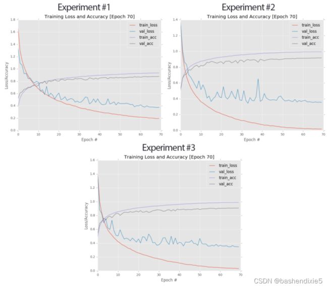左上角：实验 #1 的学习曲线。 右上角：实验#2 的图。底部：实验#3 的学习曲线。 我们的最终实验在前两者之间取得了良好的平衡，获得了 90:81% 的准确率，高于我们之前所有的 CIFAR-10 实验。

        3、Tiny ImageNet

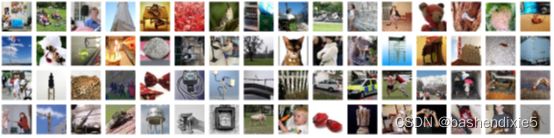来自斯坦福的 Tiny ImageNet 分类挑战的图像样本。

        3.1 下载Tiny-ImageNet

        您可以从这里的官方 cs231n 排行榜页面下载 Tiny ImageNet 数据集：
https://tiny-imagenet.herokuapp.com/https://tiny-imagenet.herokuapp.com/        .zip 文件为 237MB，因此在尝试下载之前请确保您有合理的互联网连接。

        3.2 Tiny-ImageNet 目录结构

        下载并解压 tiny-imagenet-200.zip 文件后，解压它，您会发现以下目录结构：

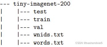
         可以通过解析 words.txt 文件来查找 WordNet ID 的人类可读标签，该文件只是一个制表符分隔的文件，第一列是 WordNet ID，第二列是人类可读的词/对象。 wnids.txt 文件列出了 ImageNet 数据集中的 200 个 WordNet ID（每行一个）。

        3.3 构建Tiny-ImageNet 数据集

        新建一个配置文件tiny_imagenet_config.py

# import the necessary packages
from os import path

# define the paths to the training and validation directories
TRAIN_IMAGES = "D:/Project/deeplearn/dataset/tiny-imagenet-200/datasets/tiny-imagenet-200/train"
VAL_IMAGES = "D:/Project/deeplearn/dataset/tiny-imagenet-200/datasets/tiny-imagenet-200/val/images"

# define the path to the file that maps validation filenames to
# their corresponding class labels
VAL_MAPPINGS = "D:/Project/deeplearn/dataset/tiny-imagenet-200/datasets/tiny-imagenet-200/val/val_annotations.txt"

# define the paths to the WordNet hierarchy files which are used
# to generate our class labels
WORDNET_IDS = "D:/Project/deeplearn/dataset/tiny-imagenet-200/datasets/tiny-imagenet-200/wnids.txt"
WORD_LABELS = "D:/Project/deeplearn/dataset/tiny-imagenet-200/datasets/tiny-imagenet-200/words.txt"

# since we do not have access to the testing data we need to
# take a number of images from the training data and use it instead
NUM_CLASSES = 200
NUM_TEST_IMAGES = 50 * NUM_CLASSES

# define the path to the output training, validation, and testing
# HDF5 files
TRAIN_HDF5 = "hdf5/train.hdf5"
VAL_HDF5 = "hdf5/val.hdf5"
TEST_HDF5 = "hdf5/test.hdf5"

# define the path to the dataset mean
DATASET_MEAN = "output/tiny-image-net-200-mean.json"

# define the path to the output directory used for storing plots,
# classification reports, etc.
OUTPUT_PATH = "output"
MODEL_PATH = path.sep.join([OUTPUT_PATH, "checkpoints/epoch_70.hdf5"])
FIG_PATH = path.sep.join([OUTPUT_PATH, "deepergooglenet_tinyimagenet.png"])
JSON_PATH = path.sep.join([OUTPUT_PATH, "deepergooglenet_tinyimagenet.json"])

        创建一个生成hdf5的文件build_tiny_imagenet.py，并运行生成hdf5文件

# import the necessary packages
import tiny_imagenet_config as config
from sklearn.preprocessing import LabelEncoder
from sklearn.model_selection import train_test_split
from customize.tools.hdf5DatasetWriter import HDF5DatasetWriter
from imutils import paths
import numpy as np
import progressbar
import json
import cv2
import os

# grab the paths to the training images, then extract the training
# class labels and encode them
trainPaths = list(paths.list_images(config.TRAIN_IMAGES))
trainLabels = [p.split(os.path.sep)[-3] for p in trainPaths]
le = LabelEncoder()
trainLabels = le.fit_transform(trainLabels)

# perform stratified sampling from the training set to construct a
# a testing set
split = train_test_split(trainPaths, trainLabels, test_size=config.NUM_TEST_IMAGES, stratify=trainLabels, random_state=42)
(trainPaths, testPaths, trainLabels, testLabels) = split

# load the validation filename => class from file and then use these
# mappings to build the validation paths and label lists
M = open(config.VAL_MAPPINGS).read().strip().split("\n")
M = [r.split("\t")[:2] for r in M]
valPaths = [os.path.sep.join([config.VAL_IMAGES, m[0]]) for m in M]
valLabels = le.transform([m[1] for m in M])

# construct a list pairing the training, validation, and testing
# image paths along with their corresponding labels and output HDF5
# files
datasets = [
 ("train", trainPaths, trainLabels, config.TRAIN_HDF5),
 ("val", valPaths, valLabels, config.VAL_HDF5),
 ("test", testPaths, testLabels, config.TEST_HDF5)]

# initialize the lists of RGB channel averages
(R, G, B) = ([], [], [])

# loop over the dataset tuples
for (dType, paths, labels, outputPath) in datasets:
    # create HDF5 writer
    print("[INFO] building {}...".format(outputPath))
    writer = HDF5DatasetWriter((len(paths), 64, 64, 3), outputPath)
    # initialize the progress bar
    widgets = ["Building Dataset: ", progressbar.Percentage(), " ", progressbar.Bar(), " ", progressbar.ETA()]
    pbar = progressbar.ProgressBar(maxval=len(paths), widgets=widgets).start()

    # loop over the image paths
    for (i, (path, label)) in enumerate(zip(paths, labels)):
        # load the image from disk
        image = cv2.imread(path)

        # if we are building the training dataset, then compute the
        # mean of each channel in the image, then update the
        # respective lists
        if dType == "train":
            (b, g, r) = cv2.mean(image)[:3]
            R.append(r)
            G.append(g)
            B.append(b)

        # add the image and label to the HDF5 dataset
        writer.add([image], [label])
        pbar.update(i)

    # close the HDF5 writer
    pbar.finish()
    writer.close()

# construct a dictionary of averages, then serialize the means to a
# JSON file
print("[INFO] serializing means...")
D = {"R": np.mean(R), "G": np.mean(G), "B": np.mean(B)}
f = open(config.DATASET_MEAN, "w")
f.write(json.dumps(D))
f.close()

        4、Tiny-ImageNet 上的 DeeperGoogLeNet

我们修改后的 GoogLeNet 架构，我们将其称为“DeeperGoogLeNet”。DeeperGoogLNet 架构与原始 GoogLeNet 架构相同，但有两个修改：（1）在第一个 CONV 层中使用了步幅为 1 1 的 5 5 个过滤器 (2) 最后两个初始模块（5a 和 5b）被排除在外。

        4.1 实施DeeperGoogLeNet

        创建deeergooglenet.py文件：

# import the necessary packages
from tensorflow.keras.layers import BatchNormalization
from tensorflow.keras.layers import Conv2D
from tensorflow.keras.layers import AveragePooling2D
from tensorflow.keras.layers import MaxPooling2D
from tensorflow.keras.layers import Activation
from tensorflow.keras.layers import Dropout
from tensorflow.keras.layers import Dense
from tensorflow.keras.layers import Flatten
from tensorflow.keras.layers import Input
from tensorflow.keras.models import Model
from tensorflow.keras.layers import concatenate
from tensorflow.keras.regularizers import l2
from tensorflow.keras import backend as K

class DeeperGoogLeNet:
    @staticmethod
    def conv_module(x, K, kX, kY, stride, chanDim, padding="same", reg=0.0005, name=None):
        # initialize the CONV, BN, and RELU layer names
        (convName, bnName, actName) = (None, None, None)

        # if a layer name was supplied, prepend it
        if name is not None:
            convName = name + "_conv"
            bnName = name + "_bn"
            actName = name + "_act"

        # define a CONV => BN => RELU pattern
        x = Conv2D(K, (kX, kY), strides=stride, padding=padding, kernel_regularizer=l2(reg), name=convName)(x)
        x = BatchNormalization(axis=chanDim, name=bnName)(x)
        x = Activation("relu", name=actName)(x)
        # return the block
        return x

    @staticmethod
    def inception_module(x, num1x1, num3x3Reduce, num3x3, num5x5Reduce, num5x5, num1x1Proj, chanDim, stage, reg=0.0005):
        # define the first branch of the Inception module which
        # consists of 1x1 convolutions
        first = DeeperGoogLeNet.conv_module(x, num1x1, 1, 1, (1, 1), chanDim, reg=reg, name=stage + "_first")

        # define the second branch of the Inception module which
        # consists of 1x1 and 3x3 convolutions
        second = DeeperGoogLeNet.conv_module(x, num3x3Reduce, 1, 1, (1, 1), chanDim, reg=reg, name=stage + "_second1")
        second = DeeperGoogLeNet.conv_module(second, num3x3, 3, 3, (1, 1), chanDim, reg=reg, name=stage + "_second2")

        # define the third branch of the Inception module which
        # are our 1x1 and 5x5 convolutions
        third = DeeperGoogLeNet.conv_module(x, num5x5Reduce, 1, 1, (1, 1), chanDim, reg=reg, name=stage + "_third1")
        third = DeeperGoogLeNet.conv_module(third, num5x5, 5, 5, (1, 1), chanDim, reg=reg, name=stage + "_third2")

        # define the fourth branch of the Inception module which
        # is the POOL projection
        fourth = MaxPooling2D((3, 3), strides=(1, 1), padding = "same", name = stage + "_pool")(x)
        fourth = DeeperGoogLeNet.conv_module(fourth, num1x1Proj, 1, 1, (1, 1), chanDim, reg = reg, name = stage + "_fourth")

        # concatenate across the channel dimension
        x = concatenate([first, second, third, fourth], axis=chanDim, name = stage + "_mixed")
        # return the block
        return x

    @staticmethod
    def build(width, height, depth, classes, reg=0.0005):
        # initialize the input shape to be "channels last" and the
        # channels dimension itself
        inputShape = (height, width, depth)
        chanDim = -1

        # if we are using "channels first", update the input shape
        # and channels dimension
        if K.image_data_format() == "channels_first":
            inputShape = (depth, height, width)
            chanDim = 1

        # define the model input, followed by a sequence of CONV =>
        # POOL => (CONV * 2) => POOL layers
        inputs = Input(shape=inputShape)
        x = DeeperGoogLeNet.conv_module(inputs, 64, 5, 5, (1, 1), chanDim, reg = reg, name = "block1")
        x = MaxPooling2D((3, 3), strides=(2, 2), padding="same", name = "pool1")(x)
        x = DeeperGoogLeNet.conv_module(x, 64, 1, 1, (1, 1), chanDim, reg = reg, name = "block2")
        x = DeeperGoogLeNet.conv_module(x, 192, 3, 3, (1, 1), chanDim, reg = reg, name = "block3")
        x = MaxPooling2D((3, 3), strides=(2, 2), padding="same", name = "pool2")(x)

        # apply two Inception modules followed by a POOL
        x = DeeperGoogLeNet.inception_module(x, 64, 96, 128, 16, 32, 32, chanDim, "3a", reg = reg)
        x = DeeperGoogLeNet.inception_module(x, 128, 128, 192, 32, 96, 64, chanDim, "3b", reg = reg)
        x = MaxPooling2D((3, 3), strides=(2, 2), padding="same", name = "pool3")(x)

        # apply five Inception modules followed by POOL
        x = DeeperGoogLeNet.inception_module(x, 192, 96, 208, 16, 48, 64, chanDim, "4a", reg = reg)
        x = DeeperGoogLeNet.inception_module(x, 160, 112, 224, 24, 64, 64, chanDim, "4b", reg = reg)
        x = DeeperGoogLeNet.inception_module(x, 128, 128, 256, 24, 64, 64, chanDim, "4c", reg = reg)
        x = DeeperGoogLeNet.inception_module(x, 112, 144, 288, 32, 64, 64, chanDim, "4d", reg = reg)
        x = DeeperGoogLeNet.inception_module(x, 256, 160, 320, 32, 128, 128, chanDim, "4e", reg = reg)
        x = MaxPooling2D((3, 3), strides=(2, 2), padding="same", name = "pool4")(x)

        # apply a POOL layer (average) followed by dropout
        x = AveragePooling2D((4, 4), name="pool5")(x)
        x = Dropout(0.4, name="do")(x)
        # softmax classifier
        x = Flatten(name="flatten")(x)
        x = Dense(classes, kernel_regularizer=l2(reg), name="labels")(x)
        x = Activation("softmax", name="softmax")(x)
        # create the model
        model = Model(inputs, x, name="googlenet")
        # return the constructed network architecture
        return model

        4.2 在Tiny-ImageNet上训练

        创建train.py

# set the matplotlib backend so figures can be saved in the background
import matplotlib
matplotlib.use("Agg")

# import the necessary packages
import tiny_imagenet_config as config
from customize.tools.imagetoarraypreprocessor import ImageToArrayPreprocessor
from customize.tools.simplepreprocessor import SimplePreprocessor
from customize.tools.meanpreprocessor import MeanPreprocessor
from tensorflow.keras.callbacks import ModelCheckpoint
from customize.tools.trainingmonitor import TrainingMonitor
from customize.tools.hdf5datasetgenerator import HDF5DatasetGenerator
from models.deepergooglenet.deeergooglenet import DeeperGoogLeNet
from tensorflow.keras.preprocessing.image import ImageDataGenerator
from tensorflow.keras.optimizers import Adam
from tensorflow.keras.models import load_model
import tensorflow.keras.backend as K
import argparse
import json

# construct the argument parse and parse the arguments
ap = argparse.ArgumentParser()
ap.add_argument("-c", "--checkpoints", required=True, help="path to output checkpoint directory")
ap.add_argument("-m", "--model", type=str, help="path to *specific* model checkpoint to load")
ap.add_argument("-s", "--start-epoch", type=int, default=0, help="epoch to restart training at")
args = vars(ap.parse_args())

# construct the training image generator for data augmentation
aug = ImageDataGenerator(rotation_range=18, zoom_range=0.15, width_shift_range=0.2,
                         height_shift_range=0.2, shear_range=0.15,
                        horizontal_flip=True, fill_mode="nearest")

# load the RGB means for the training set
means = json.loads(open(config.DATASET_MEAN).read())

# initialize the image preprocessors
sp = SimplePreprocessor(64, 64)
mp = MeanPreprocessor(means["R"], means["G"], means["B"])
iap = ImageToArrayPreprocessor()

# initialize the training and validation dataset generators
trainGen = HDF5DatasetGenerator(config.TRAIN_HDF5, 64, aug=aug, preprocessors=[sp, mp, iap], classes=config.NUM_CLASSES)
valGen = HDF5DatasetGenerator(config.VAL_HDF5, 64, preprocessors=[sp, mp, iap], classes=config.NUM_CLASSES)

# if there is no specific model checkpoint supplied, then initialize
# the network and compile the model
if args["model"] is None:
    print("[INFO] compiling model...")
    model = DeeperGoogLeNet.build(width=64, height=64, depth=3,
    classes=config.NUM_CLASSES, reg=0.0002)
    opt = Adam(1e-3)
    model.compile(loss="categorical_crossentropy", optimizer=opt, metrics=["accuracy"])
# otherwise, load the checkpoint from disk
else:
    print("[INFO] loading {}...".format(args["model"]))
    model = load_model(args["model"])

    # update the learning rate
    print("[INFO] old learning rate: {}".format(K.get_value(model.optimizer.lr)))
    K.set_value(model.optimizer.lr, 1e-5)
    print("[INFO] new learning rate: {}".format(K.get_value(model.optimizer.lr)))

# construct the set of callbacks
#callbacks = [EpochCheckpoint(args["checkpoints"], every=5, startAt=args["start_epoch"]),
#    TrainingMonitor(config.FIG_PATH, jsonPath=config.JSON_PATH, startAt=args["start_epoch"])]
model_checkpoint = ModelCheckpoint('unet_membrane.hdf5', monitor='loss', verbose=1, save_best_only=True)

# train the network
model.fit_generator(trainGen.generator(), steps_per_epoch=trainGen.numImages // 64, validation_data=valGen.generator(),
    validation_steps=valGen.numImages // 64, epochs=10, max_queue_size=64 * 2, callbacks=[model_checkpoint], verbose=1)

# close the databases
trainGen.close()
valGen.close()

        4.3 训练结果

        我决定使用 SGD 训练 DeeperGoogLenet，初始学习率为 1e-2，动量项为 0.9（未应用 Nesterov 加速）。 我总是在我的第一个实验中使用 SGD。 根据我在第 7 章中的指导方针和经验法则，您应该首先尝试 SGD 以获得基线，然后如果需要，使用更高级的优化方法。

        在 epoch 25 之后，我停止训练，将学习率降低到 1e3，然后继续训练10个epoch。

        在 epoch 35 之后，我再次停止训练，将学习率降低到 1e4，然后再继续训练 30 个 epoch。

        至少可以说，额外的 30 个 epoch 的训练是多余的。 然而，我想感受一下在原始学习率下降后预期大量 epoch 的过度拟合水平。

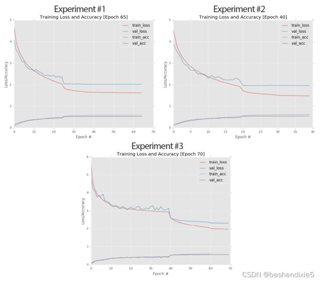左上角：实验 #1 的图。 右上角：实验#2 的学习曲线。 底部：实验#3 的训练/验证图。 最终实验在 55.77% 处获得了最佳验证准确率。

        从大约第 15 个时期开始，训练和验证损失出现分歧。当我们到达第 25 个时期时，分歧变得越来越大，所以我将学习率降低了一个数量级； 结果是准确性和损失减少了一个很好的跳跃。 问题是，在这一点之后，训练和验证学习基本上都停滞了。 即使在 epoch 35 时将学习率降低到 1e-4，也不会带来额外的准确度提升。