【机器学习】使用scikit-learn实现简单线性回归(10min左右阅读时长)
Simple Linear Regression(简单线性回归)
Objectives(目标)
看完这篇文章,将会:1.使用scikit-learn实现简单的线性回归 2.创建一个模型,训练它,测试它,并使用它
- Use scikit-learn to implement simple Linear Regression
- Create a model, train it, test it and use the model
Importing Needed packages(导入必要的包)
import matplotlib.pyplot as plt
import pandas as pd
import pylab as pl
import numpy as np
%matplotlib inline
Downloading Data(下载数据)
FuelConsumption(点我下载)
Understanding the Data(理解数据)
FuelConsumption.csv:
我们下载了一个油耗数据集, FuelConsumption.csv,其中包含了加拿大零售新轻型汽车的特定车型油耗等级和估计的二氧化碳排放量。
We have downloaded a fuel consumption dataset, FuelConsumption.csv, which contains model-specific fuel consumption ratings and estimated carbon dioxide emissions for new light-duty vehicles for retail sale in Canada. Dataset source
- MODELYEAR e.g. 2014
- MAKE e.g. Acura
- MODEL e.g. ILX
- VEHICLE CLASS e.g. SUV
- ENGINE SIZE e.g. 4.7
- CYLINDERS e.g 6
- TRANSMISSION e.g. A6
- FUEL CONSUMPTION in CITY(L/100 km) e.g. 9.9
- FUEL CONSUMPTION in HWY (L/100 km) e.g. 8.9
- FUEL CONSUMPTION COMB (L/100 km) e.g. 9.2
- CO2 EMISSIONS (g/km) e.g. 182 --> low --> 0
Reading the data in(读取数据)
# df = pd.read_csv("FuelConsumption.csv")
df=pd.read_csv("D:\MLwithPython\FuelConsumptionCo2.csv")
# 自己改个路径
# take a look at the dataset
df.head()
| MODELYEAR | MAKE | MODEL | VEHICLECLASS | ENGINESIZE | CYLINDERS | TRANSMISSION | FUELTYPE | FUELCONSUMPTION_CITY | FUELCONSUMPTION_HWY | FUELCONSUMPTION_COMB | FUELCONSUMPTION_COMB_MPG | CO2EMISSIONS | |
|---|---|---|---|---|---|---|---|---|---|---|---|---|---|
| 0 | 2014 | ACURA | ILX | COMPACT | 2.0 | 4 | AS5 | Z | 9.9 | 6.7 | 8.5 | 33 | 196 |
| 1 | 2014 | ACURA | ILX | COMPACT | 2.4 | 4 | M6 | Z | 11.2 | 7.7 | 9.6 | 29 | 221 |
| 2 | 2014 | ACURA | ILX HYBRID | COMPACT | 1.5 | 4 | AV7 | Z | 6.0 | 5.8 | 5.9 | 48 | 136 |
| 3 | 2014 | ACURA | MDX 4WD | SUV - SMALL | 3.5 | 6 | AS6 | Z | 12.7 | 9.1 | 11.1 | 25 | 255 |
| 4 | 2014 | ACURA | RDX AWD | SUV - SMALL | 3.5 | 6 | AS6 | Z | 12.1 | 8.7 | 10.6 | 27 | 244 |
Data Exploration(数据探索)
让我们首先对数据进行描述性的探索。
Let’s first have a descriptive exploration on our data.
# summarize the data
df.describe()
| MODELYEAR | ENGINESIZE | CYLINDERS | FUELCONSUMPTION_CITY | FUELCONSUMPTION_HWY | FUELCONSUMPTION_COMB | FUELCONSUMPTION_COMB_MPG | CO2EMISSIONS | |
|---|---|---|---|---|---|---|---|---|
| count | 1067.0 | 1067.000000 | 1067.000000 | 1067.000000 | 1067.000000 | 1067.000000 | 1067.000000 | 1067.000000 |
| mean | 2014.0 | 3.346298 | 5.794752 | 13.296532 | 9.474602 | 11.580881 | 26.441425 | 256.228679 |
| std | 0.0 | 1.415895 | 1.797447 | 4.101253 | 2.794510 | 3.485595 | 7.468702 | 63.372304 |
| min | 2014.0 | 1.000000 | 3.000000 | 4.600000 | 4.900000 | 4.700000 | 11.000000 | 108.000000 |
| 25% | 2014.0 | 2.000000 | 4.000000 | 10.250000 | 7.500000 | 9.000000 | 21.000000 | 207.000000 |
| 50% | 2014.0 | 3.400000 | 6.000000 | 12.600000 | 8.800000 | 10.900000 | 26.000000 | 251.000000 |
| 75% | 2014.0 | 4.300000 | 8.000000 | 15.550000 | 10.850000 | 13.350000 | 31.000000 | 294.000000 |
| max | 2014.0 | 8.400000 | 12.000000 | 30.200000 | 20.500000 | 25.800000 | 60.000000 | 488.000000 |
让我们选择一些特性来进行更多的探索。
Let’s select some features to explore more.
cdf = df[['ENGINESIZE','CYLINDERS','FUELCONSUMPTION_COMB','CO2EMISSIONS']]
cdf.head(9)
| ENGINESIZE | CYLINDERS | FUELCONSUMPTION_COMB | CO2EMISSIONS | |
|---|---|---|---|---|
| 0 | 2.0 | 4 | 8.5 | 196 |
| 1 | 2.4 | 4 | 9.6 | 221 |
| 2 | 1.5 | 4 | 5.9 | 136 |
| 3 | 3.5 | 6 | 11.1 | 255 |
| 4 | 3.5 | 6 | 10.6 | 244 |
| 5 | 3.5 | 6 | 10.0 | 230 |
| 6 | 3.5 | 6 | 10.1 | 232 |
| 7 | 3.7 | 6 | 11.1 | 255 |
| 8 | 3.7 | 6 | 11.6 | 267 |
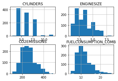
我们可以绘制出这些特征:
We can plot each of these features:
viz = cdf[['CYLINDERS','ENGINESIZE','CO2EMISSIONS','FUELCONSUMPTION_COMB']]
viz.hist()
plt.show()
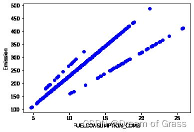
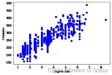
现在,让我们绘制这些特征与发射的关系,看看它们的线性关系:
Now, let’s plot each of these features against the Emission, to see how linear their relationship is:
plt.scatter(cdf.FUELCONSUMPTION_COMB, cdf.CO2EMISSIONS,  color='blue')
plt.xlabel("FUELCONSUMPTION_COMB")
plt.ylabel("Emission")
plt.show()
plt.scatter(cdf.ENGINESIZE, cdf.CO2EMISSIONS,  color='blue')
plt.xlabel("Engine size")
plt.ylabel("Emission")
plt.show()
Practice(进一步练习)
绘制CYLINDER与Emission的关系,看看它们之间的线性关系:
Plot CYLINDER vs the Emission, to see how linear is their relationship is:
plt.scatter(cdf.CYLINDERS, cdf.CO2EMISSIONS,  color='blue')
plt.xlabel("Cylinders")
plt.ylabel("Emission")
plt.show()
Creating train and test dataset(创建训练集和测试集)
训练/测试分割涉及将数据集分割为互斥的训练集和测试集。 之后,使用训练集进行训练,使用测试集进行测试。
Train/Test Split involves splitting the dataset into training and testing sets that are mutually exclusive. After which, you train with the training set and test with the testing set.
这将对样本外的准确性提供更准确的评估,因为测试数据集不是用于训练模型的数据集的一部分。 因此,它让我们更好地理解我们的模型在新数据上的泛化情况。
This will provide a more accurate evaluation on out-of-sample accuracy because the testing dataset is not part of the dataset that have been used to train the model. Therefore, it gives us a better understanding of how well our model generalizes on new data.
这意味着我们知道测试数据集中每个数据点的结果,这使得它非常适合用于测试! 由于这些数据没有被用来训练模型,所以模型不知道这些数据点的结果。 因此,从本质上讲,这是真正的样本外测试。
This means that we know the outcome of each data point in the testing dataset, making it great to test with! Since this data has not been used to train the model, the model has no knowledge of the outcome of these data points. So, in essence, it is truly an out-of-sample testing.
让我们将数据集分成训练集和测试集。 整个数据集的80%将用于训练,20%用于测试。 我们使用**np.random.rand()**函数创建一个掩码来选择随机行:
Let’s split our dataset into train and test sets. 80% of the entire dataset will be used for training and 20% for testing. We create a mask to select random rows using np.random.rand() function:
msk = np.random.rand(len(df)) < 0.8
train = cdf[msk]
test = cdf[~msk]
# msk是一串布尔值
# train就是作为训练集的那个部分
print(msk)
# print(msk)
train
[ True True True ... True True True]
| ENGINESIZE | CYLINDERS | FUELCONSUMPTION_COMB | CO2EMISSIONS | |
|---|---|---|---|---|
| 0 | 2.0 | 4 | 8.5 | 196 |
| 1 | 2.4 | 4 | 9.6 | 221 |
| 2 | 1.5 | 4 | 5.9 | 136 |
| 3 | 3.5 | 6 | 11.1 | 255 |
| 5 | 3.5 | 6 | 10.0 | 230 |
| ... | ... | ... | ... | ... |
| 1062 | 3.0 | 6 | 11.8 | 271 |
| 1063 | 3.2 | 6 | 11.5 | 264 |
| 1064 | 3.0 | 6 | 11.8 | 271 |
| 1065 | 3.2 | 6 | 11.3 | 260 |
| 1066 | 3.2 | 6 | 12.8 | 294 |
844 rows × 4 columns
Simple Regression Model(简单线性回归模型)
线性回归拟合的线性模型系数B = (B1,… , Bn)来最小化数据集中实际值y与预测值y帽之间的“残差平方和”,使用线性逼近。
Linear Regression fits a linear model with coefficients B = (B1, …, Bn) to minimize the ‘residual sum of squares’ between the actual value y in the dataset, and the predicted value yhat using linear approximation.
Train data distribution(训练集的分布)
plt.scatter(train.ENGINESIZE, train.CO2EMISSIONS,  color='blue')
plt.xlabel("Engine size")
plt.ylabel("Emission")
plt.show()
Modeling(建立模型)
Using sklearn package to model data.
from sklearn import linear_model
regr = linear_model.LinearRegression()
train_x = np.asanyarray(train[['ENGINESIZE']])
train_y = np.asanyarray(train[['CO2EMISSIONS']])
regr.fit(train_x, train_y)
# The coefficients
print ('Coefficients: ', regr.coef_)
print ('Intercept: ',regr.intercept_)
Coefficients:  [[39.92902717]]
Intercept:  [123.15528139]
如前所述,简单线性回归中的系数和截距是拟合线的参数。
As mentioned before, Coefficient and Intercept in the simple linear regression, are the parameters of the fit line.
假设它是一个简单的线性回归,只有两个参数,并且知道参数是直线的截距和斜率,sklearn可以直接从我们的数据估计它们。
Given that it is a simple linear regression, with only 2 parameters, and knowing that the parameters are the intercept and slope of the line, sklearn can estimate them directly from our data.
注意,所有数据都必须用于遍历和计算参数。(==最后用完整数据进行模型建立)
Notice that all of the data must be available to traverse and calculate the parameters.
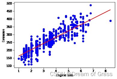
Plot outputs(结果可视化)
我们可以画一个拟合后的线
We can plot the fit line over the data:
plt.scatter(train.ENGINESIZE, train.CO2EMISSIONS,  color='blue')
plt.plot(train_x, regr.coef_[0][0]*train_x + regr.intercept_[0], '-r')
plt.xlabel("Engine size")
plt.ylabel("Emission")
Text(0, 0.5, 'Emission')
Evaluation(评估)
我们通过比较实际值和预测值来计算回归模型的准确性, 评估度量标准在模型的建立中是一个关键角色,因为它提供了对需要改进的领域的信息。
We compare the actual values and predicted values to calculate the accuracy of a regression model. Evaluation metrics provide a key role in the development of a model, as it provides insight to areas that require improvement.
这里有不同的模型评估指标,我们在这里使用MSE来计算基于测试集的模型的准确性:
There are different model evaluation metrics, lets use MSE here to calculate the accuracy of our model based on the test set:
-
Mean Absolute Error: It is the mean of the absolute value of the errors. This is the easiest of the metrics to understand since it’s just average error.
-
Mean Squared Error (MSE): Mean Squared Error (MSE) is the mean of the squared error. It’s more popular than Mean Absolute Error because the focus is geared more towards large errors. This is due to the squared term exponentially increasing larger errors in comparison to smaller ones.
-
Root Mean Squared Error (RMSE).
-
R-squared is not an error, but rather a popular metric to measure the performance of your regression model. It represents how close the data points are to the fitted regression line. The higher the R-squared value, the better the model fits your data. The best possible score is 1.0 and it can be negative (because the model can be arbitrarily worse).
from sklearn.metrics import r2_score

test_x = np.asanyarray(test[['ENGINESIZE']])
test_y = np.asanyarray(test[['CO2EMISSIONS']])
test_y_ = regr.predict(test_x)

print("Mean absolute error: %.2f" % np.mean(np.absolute(test_y_ - test_y)))
print("Residual sum of squares (MSE): %.2f" % np.mean((test_y_ - test_y) ** 2))
print("R2-score: %.2f" % r2_score(test_y , test_y_) )
Mean absolute error: 21.90
Residual sum of squares (MSE): 800.10
R2-score: 0.78
Exercise(进一步的练习)
Lets see what the evaluation metrics are if we trained a regression model using the FUELCONSUMPTION_COMB feature.
Start by selecting FUELCONSUMPTION_COMB as the train_x data from the train dataframe, then select FUELCONSUMPTION_COMB as the test_x data from the test dataframe
train_x = np.asanyarray(train[['FUELCONSUMPTION_COMB']])
test_x = test[["FUELCONSUMPTION_COMB"]]
# train_y = np.asanyarray(train[['CO2EMISSIONS']])
# train_y之前已经有了
train_x = train[["FUELCONSUMPTION_COMB"]]

test_x = test[["FUELCONSUMPTION_COMB"]]
Now train a Logistic Regression Model using the train_x you created and the train_y created previously
regr = linear_model.LinearRegression()
regr.fit(train_x, train_y)
# The coefficients
print ('Coefficients: ', regr.coef_)
print ('Intercept: ',regr.intercept_)
#ADD CODE
Coefficients:  [[16.66965333]]
Intercept:  [63.78904974]
plt.scatter(train.FUELCONSUMPTION_COMB, train.CO2EMISSIONS,  color='blue')
plt.plot(train_x, regr.coef_[0][0]*train_x + regr.intercept_[0], '-r')
plt.xlabel("FUELCONSUMPTION_COMB")
plt.ylabel("Emission")
Text(0, 0.5, 'Emission')
Find the predictions using the model’s predict function and the test_x data
predictions = regr.predict(test_x)
predictions
#ADD CODE
Finally use the predictions and the test_y data and find the Mean Absolute Error value using the np.absolute and np.mean function like done previously
#ADD CODE
# test_y = np.asanyarray(test[['CO2EMISSIONS']])
predictions = regr.predict(test_x)

print("Mean absolute error: %.2f" % np.mean(np.absolute(predictions - test_y)))
print("Residual sum of squares (MSE): %.2f" % np.mean((predictions - test_y) ** 2))
print("R2-score: %.2f" % r2_score(test_y , predictions) )
Mean absolute error: 136.65
Residual sum of squares (MSE): 20277.89
R2-score: -4.62
We can see that the MAE is much worse when we train using ENGINESIZE than FUELCONSUMPTION_COMB


