About Evaluation Metrics
you will discover how to implement four standard prediction evaluation metrics from scratch in Python.
You will know:
- How to implement classification accuracy
- How to implement and interpret a confusion matrix
- How to implement mean absolute error for regression
- How to implement root mean squared error for regression
1.1 Description
You must estimate the quality of a set of predictions when training a machine learning model.Performance metrics like classification accuracy and root mean squared error can give you a clear objective idea of how good a set of predictions is, and in turn how good the model is that generated them.This is important as it allows you to tell the difference and select among:
- Different transforms of the data used to train the same machine learning model.
- Different machine learning models trained on the same data.
- Different configurations for a machine learning model trained on the same data.
1.2 Tutorial
This tutorial is divided into 4 parts:
- Classification Accuracy
- Confusion Matrix
- Mean Absolute Error
- Root Mean Squared Error
These steps will provide the foundations you need to handle evaluating predictions made by machine learning algorithms.
1.2.1 Classification Accuracy
A quick way to evaluate a set of predictions on a classification problem is by using accuracy. Classification accuracy is a ratio of the number of correct predictions out of predictions that were made.It is often presented as a percentage between 0% for the worst possible accuracy and 100% for the best possible accuracy.
We can implement this in a function that takes the expected outcomes and the predictions as arguments.Below is this function named accuracy_metric() that returns classification accuracy as a percentage. Notice that we use == to compare the equality actual to predicted values. This allows us to compare integers or strings.two main data types that we may choose to use when loading classification data.
# Calculate accuracy percentage between two lists
def accuracy_metric(actual,predicted):
    correct = 0
    for i in range(len(actual)):
        if actual[i] == predicted[i]:
            correct += 1
    return correct / float(len(actual)) * 100.0
We can contrive a small dataset to test this function. Below are a set of 10 acutal and predicted integer values. There are two mistakes in the set of predictions.
actuall predicted
0 0
0 1
0 0
0 0
0 0
1 1
1 0
1 1
1 1
1 1
Below is a complete example with this dataset to test the accuracy_metric() function.
# Example of Calculating Classification Accuracy

# Calculate accuracy percentage between two lists
def accuracy_metric(actual, predicted):
    correct = 0
    for i in range(len(actual)):
        if actual[i] == predicted[i]:
            correct += 1
    return correct / float(len(actual)) * 100.0

# Test accuracy
actual = [0,0,0,0,0,1,1,1,1,1]
predicted = [0,1,0,0,0,1,0,1,1,1]
accuracy = accuracy_metric(actual,predicted)
print(accuracy)
Running this example produces the expected accuracy of 80% or 8/10.
Accuracy is a good metric to use when you have a small number of class values,such 2 aslo called a binary classification problem .Accuracy starts to lose it's meaning when you have more class values and you may need to review a different perspective on the results.such as a confusion matrix.
1.2.2 Confusion Matrix
A confusion matrix provides a summary of all of the predicions made compared to the expected actual values.The results are presented in a matrix with counts in each cell.The counts of predicted class values are summarized horizontally (rows), whereas the counts of actual values for each class values are presented vertically (cloumns). A perfect set of predictions is shown as a diagonal line from the top left to the bottom right of the matrix.
The value of a confusion matrix for classification problems is that you can clearly see which predictions were wrong and the type of mistake that was made.Let's create a function to calculate a confusion matrix.
We can start off by defining the function to calculate the confusion matrix given a list of actual class values and a list of predictions. The function is listed below and is named confusion_matrix(). It first makes a list of all of the unique class values and assigns each class value a unqiue integer or index into the confusion matrix.
The confusion matrix is always square, with the number of class values indicating the number of rows and columns required.Here , the first index into the matrix is the row for actual values and the second is the column for predicted values.After the square confusion matrix is created and initialized to zero counts in each cell, it is a matter of looping through all predictions and incrementing the count in each cell. The function returns two objects. The first is the set of unique class values, so that they can be displayed when the confusion matrix is drawn. The second is the confusion matrix itself with the counts in each cell.
# Function To Calculate a Confusion Matrix
# calculate a confusion matrix
def confusion_matrix(actual,predicted):
    unique = set(actual)
    matrix = [list() for x in range(len(unique))]
    for i in range(len(unique)):
        matrix[i] = [0 for x in range(len(unique))]
    lookup = dict()
    for i,value in enumerate(unique):
        lookup[value] = i
    for i in range(len(actual)):
        x = lookup[actual[i]]
        y = lookup[predicted[i]]
        matrix[y][x] += 1
    return unique,matrix
Let’s make this concrete with an example. Below is another contrived dataset, this time with 3 mistakes.
actual predicted
0 0
0 1
0 1
0 0
0 0
1 1
1 0
1 1
1 1
1 1
# Example of Calculating a Confusion Matrix

# calculate a confusion matrix
def confusion_matrix(actual,predicted):
    unique = set(actual)
    matrix = [list() for x in range(len(unique))]
    for i in range(len(unique)):
        matrix[i] = [0 for x in range(len(unique))]
    lookup = dict()
    for i,value in enumerate(unique):
        lookup = dict()
        for i ,value in enumerate(unique):
            lookup[value] = i
    for i in range(len(actual)):
        x = lookup[actual[i]]
        y = lookup[predicted[i]]
        matrix[y][x] += 1
    return unique,matrix

# Test confusion matrix with integers
actual = [0,0,0,0,0,1,1,1,1,1]
predicted = [0,1,1,0,0,1,0,1,1,1]
unique,matrix = confusion_matrix(actual,predicted)
print(unique)
print(matrix)
Running the example produces the output below. The example first prints the list of unique values and then the confusion matrix.
Below is a function to correctly display the matrix .The function is named printed_confusion_matrix().It names the columns It names the columns as Z for Actual and the rows as P for Predicted .Each column and row are named for the class value to which it corresponds.
The matrix is laid out with the expectation that each class label is a single character or single digit integer and that the counts are also single digit integers. You could extend it to handle large class labels or prediction counts as an exercise.
# Function To Pretty Print a Confusion Matrix
# pretty print a confusion matrix
def print_confusion_matrix(unique,matrix):
    print('(A)' + ' '.join(str(x) for x in unique))
    print('(P)---')
    for i, x in enumerate(unique):
        print("%s| %s " % (x, ' '.join(str(x) for x in matrix[i])))
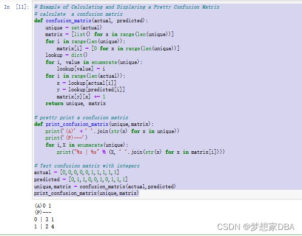
We can piece together all of the functions and display a human readable confusion matrix
# Example of Calculating and Displaying a Pretty Confusion Matrix
# calculate  a confusion matrix
def confusion_matrix(actual, predicted):
    unique = set(actual)
    matrix = [list() for x in range(len(unique))]
    for i in range(len(unique)):
        matrix[i] = [0 for x in range(len(unique))]
    lookup = dict()
    for i, value in enumerate(unique):
        lookup[value] = i
    for i in range(len(actual)):
        x = lookup[actual[i]]
        y = lookup[predicted[i]]
        matrix[y][x] += 1
    return unique, matrix

# pretty print a confusion matrix
def print_confusion_matrix(unique,matrix):
    print('(A)' + ' '.join(str(x) for x in unique))
    print('(P)---')
    for i,X in enumerate(unique):
        print("%s | %s" % (X, ' '.join(str(x) for x in matrix[i])))

# Test confusion matrix with integers
actual = [0,0,0,0,0,1,1,1,1,1]
predicted = [0,1,1,0,0,1,0,1,1,1]
unique,matrix = confusion_matrix(actual,predicted)
print_confusion_matrix(unique,matrix)
Running the example produces the output below. We can see the class labels of 0 and 1 across the top and bottom. Looking down the diagonal of the matrix from the top left to bottom right, we can see that 3 predictions of 0 were correct and 4 predictions of 1 were correct. Looking in the other cells, we can see 2 + 1 or 3 prediction errors. We can see that 2 predictions were made as a 1 that were in fact actually a 0 class value. And we can see 1 prediction that was a 0 that was in fact actually a 1.
A confusion matrix is always a good idea to use in addition to classification accuracy to help interpret the predictions.
1.2.3 Mean Absolute Error
# Calculate mean absolute error
def mae_metric(actual, predicted):
    sum_error = 0.0
    for i in range(len(actual)):
        sum_error += abs(predicted[i] - actual[i])
    return sum_error / float(len(actual))
We can contrive a small regression dataset to test this function.
actual predicted
0.1 0.11
0.2 0.19
0.3 0.29
0.4 0.41
0.5 0.5
Only one prediction (0.5) is correct, whereas all other predictions are wrong by 0.01. Therefore, we would expect the mean absolute error (or the average positive error) for these predictions to be a little less than 0.01. Below is an example that tests the mae metric() function with the contrived dataset.
# Example of Calculating Mean Absolute Error

# Calculate mean absolute error
def mae_metric(actual, predicted):
    sum_error = 0.0
    for i in range(len(actual)):
        sum_error += abs(predicted[i] - actual[i])
    return sum_error / float(len(actual))

# Test RMSE
actual = [0.1, 0.2, 0.3, 0.4, 0.5]
predicted = [0.11, 0.19, 0.29, 0.41, 0.51]
mae = mae_metric(actual,predicted)
print(mae)
Running this example prints the output below. We can see that as expected, the MAE was 0.008, a small value slightly lower than 0.01.
1.2.4 Root Mean Squared Error
# Calculate root mean squared error
def rmse_metric(actual,predicted):
    sum_error = 0.0
    for i in range(len(actual)):
        prediction_error = predicted[i] - actual[i]
        sum_error += (prediction_error ** 2)
    mean_error = sum_error / float(len(actual))
    return sqrt(mean_error)
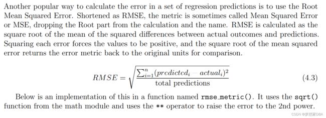
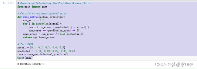
We can test this metric on the same dataset used to test the calculation of Mean Absolute Error above. Below is a complete example. Again, we would expect an error value to be generally close to 0.01.
# Example of Calculating the Root Mean Squared Error
from math import sqrt

# Calculate root mean squared error
def rmse_metric(actual,predicted):
    sum_error = 0.0
    for i in range(len(actual)):
        prediction_error = predicted[i] - actual[i]
        sum_error += (prediction_error ** 2)
    mean_error = sum_error / float(len(actual))
    return sqrt(mean_error)

# Test RMSE
actual = [0.1, 0.2, 0.3, 0.4, 0.5]
predicted = [0.11, 0.19, 0.29, 0.41, 0.5]
rmse = rmse_metric(actual,predicted)
print(rmse)
Running the example, we see the results below. The result is slightly higher at 0.0089. RMSE values are always slightly higher than MSE values, which becomes more pronounced as the prediction errors increase. This is a benefit of using RMSE over MSE in that it penalizes larger errors with worse scores.


