pytorch实现手写数字识别_LeNet-5网络实现手写数字识别

LeNet-5是经典CNN（Convolutional Neural Network）神经网络构造之一，第一次是在1995年由 Yann LeCun, Leon Bottou, Yoshua Bengio, 和 Patrick Haffner提出的，这种神经网络结构在MINIST手写数字数据集上取得了优异的结果。下面将与LeNet-5的相关知识介绍一下。

前馈神经网络的限制

当前流行的神经网络主要有三种，前馈神经网络、卷积神经网络和循环神经网络。前馈神经网络是最经典的网络模型，根据通用近似原理，前馈神经网络可以拟合所有的复杂函数，同样也可以用于图像相关的神经网络模型。但是前馈神经网络运用在图像中存在一下几点限制：

• 图像构成的数据，数据维度极大，造成前馈神经网络参数极多，达到数亿级别，虽然计算机计算速度较快，但是面对这种级别的参数学习，仍然力不从心。
• 图像数据输入前馈神经网络时，需要将图片展开为一列，这会导致原本相邻的像素点信息，展开之后距离极远，会导致神经网络对图像的学习不理想，忽略了原本的图像位置关系。
• 图像有些不变特征。比如图像经过放大，缩小，剪切之后，图像大体样貌不变。前馈神经网络处理图像时，这些不变的特性并没有得到很好的利用。

卷积神经网络特点

卷积神经网络可以很好的解决前馈神经网络面对的问题，关键点在于卷积神经网络的独特结构。

卷积神经网络是一种改善的前馈神经网络，也通过反向传播算法进行学习。卷积神经网络的特点是：

• 参数共享（Parameter sharing）：一个特征检测器，适用于图片的所有部分。
• 稀疏连接（Sparsity of connections）：每层的输出值依赖于输出值的一部分。

LeNet-5

LeNet-5是最早出现的卷积神经网络，推动了卷积神经网络的迅速发展。

LeNet-5包含七层，不包括输入，每一层都包含可训练参数。一个最典型的LeNet-5神经网络模型如下图所示，

模型包含卷积层，池化层和全连接层，上图实例输入图片是32*32像素大小，实际上MINIST图片大小为28*28大小。因此对这个模型做一点点改动。

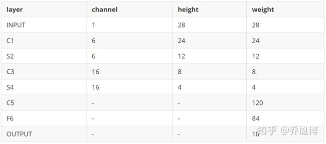
经过这样的改造，就可以完美适配本次实验的数据集。

MINIST数据集的读取

之前的文章中从零开始实现神经网络--基于MINIST手写数字数据集，有对这个手写数字数据集的介绍，这里和之前有一点点不同，就是测试集的label不需要one-hot形式，而直接采用数字结果即可。

def data_fetch_preprocessing():
    train_image = open('train-images.idx3-ubyte', 'rb')
    test_image = open('t10k-images.idx3-ubyte', 'rb')
    train_label = open('train-labels.idx1-ubyte', 'rb')
    test_label = open('t10k-labels.idx1-ubyte', 'rb')

    magic, n = struct.unpack('>II',
                             train_label.read(8))
    # 原始数据的标签
    y_train_label = np.array(np.fromfile(train_label,
                                         dtype=np.uint8), ndmin=1)
    y_train = np.ones((10, 60000)) * 0.01
    for i in range(60000):
        y_train[y_train_label[i]][i] = 0.99

    # 测试数据的标签
    magic_t, n_t = struct.unpack('>II',
                                 test_label.read(8))
    y_test = np.fromfile(test_label,
                         dtype=np.uint8).reshape(10000, 1)
    # print(y_train[0])
    # 训练数据共有60000个
    # print(len(labels))
    magic, num, rows, cols = struct.unpack('>IIII', train_image.read(16))
    x_train = np.fromfile(train_image, dtype=np.uint8).reshape(len(y_train_label), 784)

    magic_2, num_2, rows_2, cols_2 = struct.unpack('>IIII', test_image.read(16))
    x_test = np.fromfile(test_image, dtype=np.uint8).reshape(len(y_test), 784)
    # print(x_train.shape)
    # 可以通过这个函数观察图像
    # data=x_train[:,0].reshape(28,28)
    # plt.imshow(data,cmap='Greys',interpolation=None)
    # plt.show()

    # 关闭打开的文件
    train_image.close()
    train_label.close()
    test_image.close()
    test_label.close()

    return x_train, y_train_label, x_test, y_test

建立模型

本次实战采用pytorch构建模型，并进行训练，和更新参数。

class convolution_neural_network(nn.Module):
    def __init__(self):
        super(convolution_neural_network, self).__init__()

        # 定义卷积层
        self.conv = nn.Sequential(
            nn.Conv2d(in_channels=1, out_channels=6, kernel_size=5, stride=1, padding=0),  # 28x28x1-->24x24x6
            nn.Sigmoid(),
            nn.MaxPool2d(kernel_size=2, stride=2),  # 12x12x6
            nn.Conv2d(in_channels=6, out_channels=16, kernel_size=5, stride=1, padding=0),  # 8x8x16
            nn.Sigmoid(),
            nn.MaxPool2d(kernel_size=2, stride=2)  # 4x4x16
        )
        # 定义全连接层
        self.fc = nn.Sequential(
            nn.Linear(in_features=256, out_features=120),
            nn.Sigmoid(),
            nn.Linear(in_features=120, out_features=84),
            nn.Sigmoid(),
            nn.Linear(in_features=84, out_features=10),
        )
    # 前向传播过程
    def forward(self, img):
        feature = self.conv(img)
        output = self.fc(feature.view(img.shape[0], -1))
        return output

运行模型

运行模型，采用随机梯度下降的方法来更新参数，实验中设置5轮次的迭代，最终得到超过0.98的正确率。

if __name__ == '__main__':
    # 获取数据
    x_train, y_train, x_test, y_test = data_fetch_preprocessing()
    x_train = x_train.reshape(60000, 1, 28, 28)
    # 建立模型实例
    LeNet = convolution_neural_network()
    # plt.imshow(x_train[2][0], cmap='Greys', interpolation=None)
    # plt.show()
    # 交叉熵损失函数
    loss_function = nn.CrossEntropyLoss()
    loss_list = []
    optimizer = optim.Adam(params=LeNet.parameters(), lr=0.001)
    # epoch = 5
    for e in range(5):
        precision = 0
        for i in range(60000):
            prediction = LeNet(torch.tensor(x_train[i]).float().reshape(-1, 1, 28, 28))
            # print(prediction)
            # print(torch.from_numpy(y_train[i]).reshape(1,-1))
            # exit(-1)
            if torch.argmax(prediction) == y_train[i]:
                precision += 1
            loss = loss_function(prediction, torch.tensor([y_train[i]]).long())
            optimizer.zero_grad()
            loss.backward()
            optimizer.step()
            loss_list.append(loss)
        print('第%d轮迭代，loss=%.3f，准确率：%.3f' % (e, loss_list[-1],precision/60000))

总结

经过实战LeNet-5确实对手写数字数据集有效，并能取得不错的识别结果。

附录 完整代码

#!/usr/bin/env python
# -*- coding:utf-8 -*-
# File: lenet.py
# datetime: 2020/8/7 21:24
# software: PyCharm

import torch.nn as nn
import torch
import torch.optim as optim
import numpy as np
import struct
import matplotlib.pyplot as plt


def data_fetch_preprocessing():
    train_image = open('train-images.idx3-ubyte', 'rb')
    test_image = open('t10k-images.idx3-ubyte', 'rb')
    train_label = open('train-labels.idx1-ubyte', 'rb')
    test_label = open('t10k-labels.idx1-ubyte', 'rb')

    magic, n = struct.unpack('>II',
                             train_label.read(8))
    # 原始数据的标签
    y_train_label = np.array(np.fromfile(train_label,
                                         dtype=np.uint8), ndmin=1)
    y_train = np.ones((10, 60000)) * 0.01
    for i in range(60000):
        y_train[y_train_label[i]][i] = 0.99

    # 测试数据的标签
    magic_t, n_t = struct.unpack('>II',
                                 test_label.read(8))
    y_test = np.fromfile(test_label,
                         dtype=np.uint8).reshape(10000, 1)
    # print(y_train[0])
    # 训练数据共有60000个
    # print(len(labels))
    magic, num, rows, cols = struct.unpack('>IIII', train_image.read(16))
    x_train = np.fromfile(train_image, dtype=np.uint8).reshape(len(y_train_label), 784)

    magic_2, num_2, rows_2, cols_2 = struct.unpack('>IIII', test_image.read(16))
    x_test = np.fromfile(test_image, dtype=np.uint8).reshape(len(y_test), 784)
    # print(x_train.shape)
    # 可以通过这个函数观察图像
    # data=x_train[:,0].reshape(28,28)
    # plt.imshow(data,cmap='Greys',interpolation=None)
    # plt.show()

    # 关闭打开的文件
    train_image.close()
    train_label.close()
    test_image.close()
    test_label.close()

    return x_train, y_train_label, x_test, y_test


class convolution_neural_network(nn.Module):
    def __init__(self):
        super(convolution_neural_network, self).__init__()

        # 定义卷积层
        self.conv = nn.Sequential(
            nn.Conv2d(in_channels=1, out_channels=6, kernel_size=5, stride=1, padding=0),  # 28x28x1-->24x24x6
            nn.Sigmoid(),
            nn.MaxPool2d(kernel_size=2, stride=2),  # 12x12x6
            nn.Conv2d(in_channels=6, out_channels=16, kernel_size=5, stride=1, padding=0),  # 8x8x16
            nn.Sigmoid(),
            nn.MaxPool2d(kernel_size=2, stride=2)  # 4x4x16
        )
        self.fc = nn.Sequential(
            nn.Linear(in_features=256, out_features=120),
            nn.Sigmoid(),
            nn.Linear(in_features=120, out_features=84),
            nn.Sigmoid(),
            nn.Linear(in_features=84, out_features=10),
        )

    def forward(self, img):
        feature = self.conv(img)
        output = self.fc(feature.view(img.shape[0], -1))
        return output


if __name__ == '__main__':
    # 获取数据
    x_train, y_train, x_test, y_test = data_fetch_preprocessing()
    x_train = x_train.reshape(60000, 1, 28, 28)
    # 建立模型实例
    LeNet = convolution_neural_network()
    # plt.imshow(x_train[2][0], cmap='Greys', interpolation=None)
    # plt.show()
    # 交叉熵损失函数
    loss_function = nn.CrossEntropyLoss()
    loss_list = []
    optimizer = optim.Adam(params=LeNet.parameters(), lr=0.001)
    # epoch = 5
    for e in range(5):
        precision = 0
        for i in range(60000):
            prediction = LeNet(torch.tensor(x_train[i]).float().reshape(-1, 1, 28, 28))
            # print(prediction)
            # print(torch.from_numpy(y_train[i]).reshape(1,-1))
            # exit(-1)
            if torch.argmax(prediction) == y_train[i]:
                precision += 1
            loss = loss_function(prediction, torch.tensor([y_train[i]]).long())
            optimizer.zero_grad()
            loss.backward()
            optimizer.step()
            loss_list.append(loss)
        print('第%d轮迭代，loss=%.3f，准确率：%.3f' % (e, loss_list[-1],precision/60000))