眼底图像血管增强与分割--（5）基于Hessian矩阵的Frangi滤波算法

在最优化里面提到过的hessian矩阵（http://blog.csdn.net/piaoxuezhong/article/details/60135153），本篇讲的方法主要是基于Hessian矩阵实现血管边缘增强的，所以再来看一遍Hessian矩阵：

Hessian矩阵：

在数学中，Hessian矩阵是标量函数的二阶偏导数的平方矩阵。它描述了一个多变量函数的局部曲率，其基本形式为：

 

对于一副图像 I 而言，它只有x，y两个方向，所以其Hessian矩阵是一个二元矩阵，对应的有：

分别对图像卷积运算，然后构成图像Hessian矩阵：

由于二阶偏导数对噪声比较敏感，所以在求Hessian矩阵时先进行高斯平滑，对应的matlab实现：

 

function [Dxx,Dxy,Dyy] = Hessian2D(I,Sigma)  
% inputs,  
%   I : The image, class preferable double or single  
%   Sigma : The sigma of the gaussian kernel used  
%  
% outputs,  
%   Dxx, Dxy, Dyy: The 2nd derivatives  
  
if nargin < 2, Sigma = 1; end  
  
% Make kernel coordinates  
[X,Y]   = ndgrid(-round(Sigma):round(Sigma));  
  
% Build the gaussian 2nd derivatives filters  
DGaussxx = 1/(2*pi*Sigma^4) * (X.^2/Sigma^2 - 1) .* exp(-(X.^2 + Y.^2)/(2*Sigma^2));  
DGaussxy = 1/(2*pi*Sigma^6) * (X .* Y).* exp(-(X.^2 + Y.^2)/(2*Sigma^2));  
DGaussyy = 1/(2*pi*Sigma^4) * (Y.^2/Sigma^2 - 1) .* exp(-(X.^2 + Y.^2)/(2*Sigma^2));  
  
Dxx = imfilter(I,DGaussxx,'conv');  
Dxy = imfilter(I,DGaussxy,'conv');  
Dyy = imfilter(I,DGaussyy,'conv');  

测试函数：

 

 

%% EST hessian  
clc;close all;clear all;  
I=imread ('D:\fcq_proMatlab\test_image\retina\9.jpg');  
I=double(rgb2gray(I));  
[Dxx,Dxy,Dyy] = Hessian2D(I,.3);  
figure,  
subplot(211), imshow(I,[]);title('original image');  
subplot(212), imshow(Dxx,[]);title('hessian Dxx image');  

 

Frangi滤波：

 

Frangi滤波分为二维和三维两种情况，这里只说Frangi2D滤波。Frangi滤波是基于Hessian矩阵构造出来的一种边缘检测增强滤波算法。
（3）

在上面的Hessian程序中，高斯平滑参数σ为标准差，对于血管这种线形结构，当尺度因子 σ 与血管的实际宽度最匹配时，滤波器的输出最大。所以作为空间尺度因子，迭代可以得到不同尺度的输出。局部特性分析的窗口矩形的半宽一般为 3σ。血管直径小于当前尺度相应的窗口矩形的宽和高时，管状血管的 Hessian 矩阵的特征值满足: | λ1| ≈0， |λ1| ＜ ＜ | λ2| 。用λ1和λ2定义R,S特征值：

 

增补：

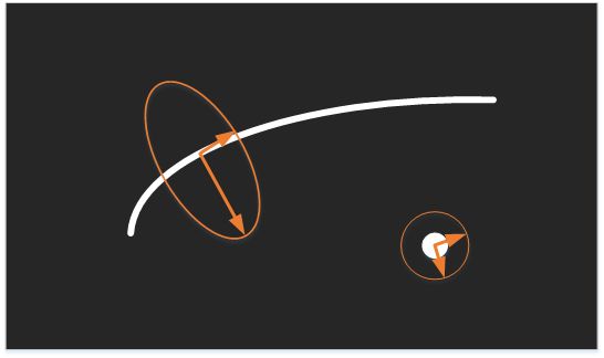
在二维图像中，海森矩阵是二维正定矩阵，有两个特征值和对应的两个特征向量。两个特征值表示出了图像在两个特征向量所指方向上图像变化的各向异性。在二维图像中，圆具有最强的各项同性，线性越强的结构越具有各向异性。

且特征值应该具有如下特性；

λ1	λ2	图像特征
-High	-High	斑点结构（前景为亮）
+High	+High	斑点结构（前景为暗）
Low	-High	线性结构（前景为亮）
Low	+High	线性结构（前景为暗）

下面是作者的方法实现，对照程序和论文，算法步骤就比较清楚了：

(1)FrangiFilter2D函数
function [outIm,whatScale,Direction] = FrangiFilter2D(I, options)  
% This function FRANGIFILTER2D uses the eigenvectors of the Hessian to  
% compute the likeliness of an image region to vessels, according  
% to the method described by Frangi:2001 (Chapter 2).  
% [J,Scale,Direction] = FrangiFilter2D(I, Options)  
% inputs,  
%   I : The input image (vessel image)  
%   Options : Struct with input options,  
%       .FrangiScaleRange : The range of sigmas used, default [1 8]  
%       .FrangiScaleRatio : Step size between sigmas, default 2  
%       .FrangiBetaOne : Frangi correction constant, default 0.5  
%       .FrangiBetaTwo : Frangi correction constant, default 15  
%       .BlackWhite : Detect black ridges (default) set to true, for  
%                       white ridges set to false.  
%       .verbose : Show debug information, default true  
% outputs,  
%   J : The vessel enhanced image (pixel is the maximum found in all scales)  
%   Scale : Matrix with the scales on which the maximum intensity   
%           of every pixel is found  
%   Direction : Matrix with directions (angles) of pixels (from minor eigenvector)     
%  
% Written by Marc Schrijver, 2/11/2001  
% Re-Written by D.Kroon University of Twente (May 2009)  
  
defaultoptions = struct('FrangiScaleRange', [1 10], 'FrangiScaleRatio', 2, 'FrangiBetaOne', 0.5, 'FrangiBetaTwo', 15, 'verbose',true,'BlackWhite',true);  
  
% Process inputs  
if(~exist('options','var')),   
    options=defaultoptions;   
else  
    tags = fieldnames(defaultoptions);  
    for i=1:length(tags)  
         if(~isfield(options,tags{i})),  options.(tags{i})=defaultoptions.(tags{i}); end  
    end  
    if(length(tags)~=length(fieldnames(options))),   
        warning('FrangiFilter2D:unknownoption','unknown options found');  
    end  
end  
  
%sigam范围从FrangiScaleRange（1）到FrangiScaleRange（2），步长为FrangiScaleRatio，具体要结合图像  
  
sigmas=options.FrangiScaleRange(1):options.FrangiScaleRatio:options.FrangiScaleRange(2);  
sigmas = sort(sigmas, 'ascend');  
  
beta  = 2*options.FrangiBetaOne^2;  
c     = 2*options.FrangiBetaTwo^2;  
  
% Make matrices to store all filterd images  
ALLfiltered=zeros([size(I) length(sigmas)]);  
ALLangles=zeros([size(I) length(sigmas)]);  
  
% Frangi filter for all sigmas  
for i = 1:length(sigmas),  
    % Show progress  
    if(options.verbose)  
        disp(['Current Frangi Filter Sigma: ' num2str(sigmas(i)) ]);  
    end  
      
    % Make 2D hessian  
    [Dxx,Dxy,Dyy] = Hessian2D(I,sigmas(i));  
      
    % Correct for scale  
    Dxx = (sigmas(i)^2)*Dxx;  
    Dxy = (sigmas(i)^2)*Dxy;  
    Dyy = (sigmas(i)^2)*Dyy;  
     
    % Calculate (abs sorted) eigenvalues and vectors  
    [Lambda2,Lambda1,Ix,Iy]=eig2image(Dxx,Dxy,Dyy);  
  
    % Compute the direction of the minor eigenvector  
    angles = atan2(Ix,Iy);  
  
    % Compute some similarity measures  
    Lambda1(Lambda1==0) = eps;  
    Rb = (Lambda2./Lambda1).^2;  
    S2 = Lambda1.^2 + Lambda2.^2;  
     
    % Compute the output image  
    Ifiltered = exp(-Rb/beta) .*(ones(size(I))-exp(-S2/c));  
      
    % see pp. 45  
    if(options.BlackWhite)  
        Ifiltered(Lambda1<0)=0;  
    else  
        Ifiltered(Lambda1>0)=0;  
    end  
    % store the results in 3D matrices  
    ALLfiltered(:,:,i) = Ifiltered;  
    ALLangles(:,:,i) = angles;  
end  
  
% Return for every pixel the value of the scale(sigma) with the maximum   
% output pixel value  
if length(sigmas) > 1,  
    [outIm,whatScale] = max(ALLfiltered,[],3);  
    outIm = reshape(outIm,size(I));  
    if(nargout>1)  
        whatScale = reshape(whatScale,size(I));  
    end  
    if(nargout>2)  
        Direction = reshape(ALLangles((1:numel(I))'+(whatScale(:)-1)*numel(I)),size(I));  
    end  
else  
    outIm = reshape(ALLfiltered,size(I));  
    if(nargout>1)  
            whatScale = ones(size(I));  
    end  
    if(nargout>2)  
        Direction = reshape(ALLangles,size(I));  
    end  
end  

（2）Hessian2D函数
function [Dxx,Dxy,Dyy] = Hessian2D(I,Sigma)
%  This function Hessian2 Filters the image with 2nd derivatives of a 
%  Gaussian with parameter Sigma.
% 
% [Dxx,Dxy,Dyy] = Hessian2(I,Sigma);
% 
% inputs,
%   I : The image, class preferable double or single
%   Sigma : The sigma of the gaussian kernel used
%
% outputs,
%   Dxx, Dxy, Dyy: The 2nd derivatives
%
% example,
%   I = im2double(imread('moon.tif'));
%   [Dxx,Dxy,Dyy] = Hessian2(I,2);
%   figure, imshow(Dxx,[]);
%
% Function is written by D.Kroon University of Twente (June 2009)

if nargin < 2, Sigma = 1; end

% Make kernel coordinates
[X,Y]   = ndgrid(-round(3*Sigma):round(3*Sigma));

% Build the gaussian 2nd derivatives filters
DGaussxx = 1/(2*pi*Sigma^4) * (X.^2/Sigma^2 - 1) .* exp(-(X.^2 + Y.^2)/(2*Sigma^2));
DGaussxy = 1/(2*pi*Sigma^6) * (X .* Y)           .* exp(-(X.^2 + Y.^2)/(2*Sigma^2));
DGaussyy = DGaussxx';

Dxx = imfilter(I,DGaussxx,'conv');
Dxy = imfilter(I,DGaussxy,'conv');
Dyy = imfilter(I,DGaussyy,'conv');
% Dxx = imfilter(I,DGaussxx);
% Dxy = imfilter(I,DGaussxy);
% Dyy = imfilter(I,DGaussyy);
end

（3）eig2image函数
function [Lambda1,Lambda2,Ix,Iy]=eig2image(Dxx,Dxy,Dyy)
% This function eig2image calculates the eigen values from the
% hessian matrix, sorted by abs value. And gives the direction
% of the ridge (eigenvector smallest eigenvalue) .
% 
% [Lambda1,Lambda2,Ix,Iy]=eig2image(Dxx,Dxy,Dyy)
%
%
% | Dxx  Dxy |
% |          |
% | Dxy  Dyy |
% Compute the eigenvectors of J, v1 and v2
tmp = sqrt((Dxx - Dyy).^2 + 4*Dxy.^2);
v2x = 2*Dxy; v2y = Dyy - Dxx + tmp;

% Normalize
mag = sqrt(v2x.^2 + v2y.^2); i = (mag ~= 0);
v2x(i) = v2x(i)./mag(i);
v2y(i) = v2y(i)./mag(i);

% The eigenvectors are orthogonal
v1x = -v2y; 
v1y = v2x;

% Compute the eigenvalues
mu1 = 0.5*(Dxx + Dyy + tmp);
mu2 = 0.5*(Dxx + Dyy - tmp);

% Sort eigen values by absolute value abs(Lambda1)abs(mu2);

Lambda1=mu1; Lambda1(check)=mu2(check);
Lambda2=mu2; Lambda2(check)=mu1(check);

Ix=v1x; Ix(check)=v2x(check);
Iy=v1y; Iy(check)=v2y(check);

下面这幅图像我设置的sigam参数就是（0.05:0.05：5），测试函数为：

%% TEST Frangi_filter  
clc;close all;clear all;  
I=imread ('D:\fcq_proMatlab\test_image\retina\13.jpg');  
I=double(rgb2gray(I));  
Ivessel=FrangiFilter2D(I);  
figure,  
subplot(1,2,1), imshow(I,[]);title('原灰度图');  
subplot(1,2,2), imshow(Ivessel,[]);title('Frangi滤波结果')  

 

参考：

• https://en.wikipedia.org/wiki/Hessian_matrix

• 《Multiscale vessel enhancement filtering》[C]. International Conference on Medical Image Computing & Computer-assisted Intervention

• http://blog.csdn.net/u013288466/article/details/73648757
• 《肺部CT图像血管分割算法与三维可视化的研究》[J].
• 《基于 Hessian 算子的多尺度视网膜血管增强滤波方法》[J].计算机应用与软件
• https://blog.csdn.net/dfdfdsfdfdfdf/article/details/81019927
• https://ww2.mathworks.cn/matlabcentral/fileexchange/24409-hessian-based-frangi-vesselness-filter?requestedDomain=zh