als pyspark
Recommender System is an information filtering tool that seeks to predict which product a user will like, and based on that, recommends a few products to the users. For example, Amazon can recommend new shopping items to buy, Netflix can recommend new movies to watch, and Google can recommend news that a user might be interested in. The two widely used approaches for building a recommender system are the content-based filtering (CBF) and collaborative filtering (CF).
推荐系统是一种信息过滤工具,旨在预测用户喜欢的产品,并在此基础上向用户推荐一些产品。 例如,亚马逊可以推荐要购买的新购物商品,Netflix可以推荐要观看的新电影,Google可以推荐用户可能感兴趣的新闻。构建推荐系统的两种广泛使用的方法是基于内容的过滤( CBF)和协作过滤(CF)。
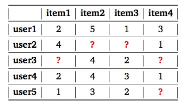
To understand the concept of recommender systems, let us look at an example. The below table shows the user-item utility matrix Y where the value Rui denotes how item i has been rated by user u on a scale of 1–5. The missing entries (shown by ? in Table) are the items that have not been rated by the respective user.
为了理解推荐系统的概念,让我们看一个例子。 下表显示了用户项效用矩阵 Y,其中Rui值表示用户i如何以1-5的等级对项i进行评分。 缺少的条目(在表中用?显示)是尚未由相应用户评分的项目。
utility matrix 效用矩阵The objective of the recommender system is to predict the ratings for these items. Then the highest rated items can be recommended to the respective users. In real world problems, the utility matrix is expected to be very sparse, as each user only encounters a small fraction of items among the vast pool of options available. The code for this project can be found here.
推荐系统的目的是预测这些项目的评级。 然后可以向各个用户推荐评分最高的项目。 在现实世界中,效用矩阵非常稀疏,因为每个用户在大量可用选项中仅会遇到一小部分项目。 该项目的代码可以在这里找到。
显式与隐式评级 (Explicit v.s. Implicit ratings)
There are two ways to gather user preference data to recommend items, the first method is to ask for explicit ratings from a user, typically on a concrete rating scale (such as rating a movie from one to five stars) making it easier to make extrapolations from data to predict future ratings. However, the drawback with explicit data is that it puts the responsibility of data collection on the user, who may not want to take time to enter ratings. On the other hand, implicit data is easy to collect in large quantities without any extra effort on the part of the user. Unfortunately, it is much more difficult to work with.
有两种收集用户偏好数据以推荐项目的方法,第一种方法是要求用户提供明确的评级 ,通常以具体的评级标准(例如,将电影从一星评级为五颗星)进行推断就容易了。从数据中预测未来的收视率。 但是,显式数据的缺点是将数据收集的责任交给了用户,而用户可能不想花时间输入评分。 另一方面, 隐式数据易于大量收集,而无需用户付出任何额外的努力。 不幸的是,要处理它要困难得多。
数据稀疏和冷启动 (Data Sparsity and Cold Start)
In real world problems, the utility matrix is expected to be very sparse, as each user only encounters a small fraction of items among the vast pool of options available. Cold-Start problem can arise during addition of a new user or a new item where both do not have history in terms of ratings. Sparsity can be calculated using the below function.
在现实世界中,效用矩阵非常稀疏,因为每个用户在大量可用选项中只遇到一小部分项目。 在添加新用户或新项目时,如果两者都没有评级历史记录,则会出现冷启动问题。 稀疏度可以使用以下函数来计算。
1.具有显式评分的数据集(MovieLens) (1. Dataset with Explicit Ratings (MovieLens))
MovieLens is a recommender system and virtual community website that recommends movies for its users to watch, based on their film preferences using collaborative filtering. MovieLens 100M datatset is taken from the MovieLens website, which customizes user recommendation based on the ratings given by the user. To understand the concept of recommendation system better, we will work with this dataset. This dataset can be downloaded from here.
MovieLens是一个推荐器系统和虚拟社区网站,它根据用户使用协作筛选的电影偏好来推荐电影供其观看。 MovieLens 100M数据集来自MovieLens网站,该网站根据用户给出的等级来自定义用户推荐。 为了更好地理解推荐系统的概念,我们将使用此数据集。 可以从此处下载该数据集。
There are 2 tuples, movies and ratings which contains variables such as MovieID::Genre::Title and UserID::MovieID::Rating::Timestamp respectively.
有2个元组,电影和等级,其中分别包含MovieID :: Genre :: Title和UserID :: MovieID :: Rating :: Timestamp等变量。
Let’s load the data and explore the data. To load the data as a spark dataframe, import pyspark and instantiate a spark session.
让我们加载数据并浏览数据。 要将数据加载为spark数据框,请导入pyspark并实例化spark会话。
from pyspark.sql import SparkSession
spark = SparkSession.builder.appName('Recommendations').getOrCreate()movies = spark.read.csv("movies.csv",header=True)
ratings = spark.read.csv("ratings.csv",header=True)
ratings.show()# Join both the data frames to add movie data into ratings
movie_ratings = ratings.join(movies, ['movieId'], 'left')
movie_ratings.show()Lets calculate the data sparsity to understand the sparsity of the data. Please function that we built in the begining of this article to get the sparsity. The movie lens data is 98.36% sparse.
让我们计算数据稀疏性以了解数据稀疏性。 请发挥我们在本文开头构建的功能以获得稀疏性。 电影镜头数据为98.36%稀疏。
get_mat_sparsity(ratings)Before moving into recommendations, split the dataset into train and test. Please set the seed to reproduce results. We will look at different recommendation techniques in detail in the below sections.
在提出建议之前,请将数据集分为训练和测试。 请设置种子以重现结果。 我们将在以下各节中详细介绍不同的推荐技术。
# Create test and train set
(train, test) = ratings.randomSplit([0.8, 0.2], seed = 2020)
2.具有二进制等级的数据集(MovieLens) (2. Dataset with Binary Ratings (MovieLens))
With some datasets, we don’t have the luxury to work with explicit ratings. For those datasets we must infer ratings from the given information. In MovieLens dataset, let us add implicit ratings using explicit ratings by adding 1 for watched and 0 for not watched. We aim the model to give high predictions for movies watched.
对于某些数据集,我们没有足够的精力进行明确的评分。 对于这些数据集,我们必须根据给定的信息推断等级。 在MovieLens数据集中,让我们使用显式评级添加隐式评级,方法是将观看次数增加1,将未观看次数增加0。 我们的模型旨在为观看的电影提供较高的预测。
Please note this is not the right dataset for implict ratings since there may be movies in the not watched set, which the user has actually watched but not given a rating.
请注意,这不是隐式收视率的正确数据集,因为可能有未观看集中的电影,这些电影是用户实际看过但未给出收视率的。
user_movie.show()推荐方法 (Approaches to Recommendation)
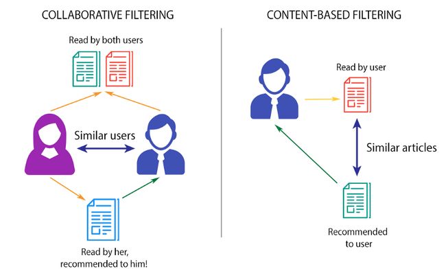
The two widely used approaches for building a recommender system are the content-based filtering (CBF) and collaborative filtering (CF), of which CBF is the most widely used. The below figure illustrates the concepts of CF and CBF. The primary difference between these two approaches is that CF looks for similar users to recommend items while CBF looks for similar contents to recommend items.
建立推荐系统的两种广泛使用的方法是基于内容的过滤(CBF)和协作过滤(CF),其中CBF使用最广泛。 下图说明了CF和CBF的概念。 这两种方法之间的主要区别在于,CF寻找相似的用户来推荐商品,而CBF寻找相似的内容来推荐商品。
协同过滤(CF) (Collaborative filtering (CF))
Collaborative filtering aggregates the past behaviour of all users. It recommends items to a user based on the items liked by another set of users whose likes (and dislikes) are similar to the user under consideration. This approach is also called the user-user based CF.
协作过滤汇总了所有用户的过去行为。 它基于喜欢(和不喜欢)与正在考虑的用户相似的另一组用户喜欢的项目,向用户推荐项目。 这种方法也称为基于用户-用户的CF。
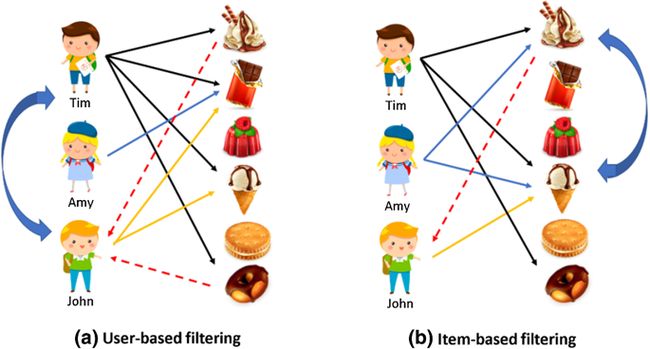
item-item based CF became popular later, where to recommend an item to a user, the similarity between items liked by the user and other items are calculated. The user-user CF and item-item CF can be achieved by two different ways, memory-based (neighbourhood approach) and model-based (latent factor model approach).
基于项目的CF后来变得很流行,向用户推荐项目,计算用户喜欢的项目与其他项目之间的相似度。 用户-用户CF和项目CF可以通过两种不同的方式来实现:基于内存的 (邻域方法)和基于模型的 (潜在因子模型方法)。
1.基于内存的(邻域方法) (1. The memory-based (neighbourhood approach))
To recommend items to user u1 in the user-user based neighborhood approach first a set of users whose likes and dislikes similar to the useru1 is found using a similarity metrics which captures the intuition that sim(u1, u2) >sim(u1, u3) where user u1 and u2 are similar and user u1 and u3 are dissimilar. similar user is called the neighbourhood of user u1.
为了在基于用户-用户的邻域方法中向用户u1推荐商品,首先使用相似度指标找到一组与useru1相似的好恶的用户,这些相似性指标可捕捉sim(u1,u2)> sim(u1,u3)的直觉),其中用户u1和u2是相似的,而用户u1和u3是不相似的。 类似的用户称为用户u1的邻居。
Image credit 图片信用Neighbourhood approaches are most effective at detecting very localized relationships (neighbours), ignoring other users. But the downsides are that, first, the data gets sparse which hinders scalability, and second, they perform poorly in terms of reducing the RMSE (root-mean-squared-error) compared to other complex methods.
邻域方法最有效地检测非常本地化的关系(邻域),而忽略其他用户。 但是缺点是,首先,数据稀疏,这阻碍了可伸缩性,其次,与其他复杂方法相比,它们在减少RMSE(均方根误差)方面表现不佳。
2.基于模型(潜在因子模型方法) (2. The model-based (latent factor model approach))
Latent factor model based collaborative filtering learns the (latent) user and item profiles (both of dimension K) through matrix factorization by minimizing the RMSE (Root Mean Square Error) between the available ratings yand their predicted values yˆ. Here each item i is associated with a latent (feature) vector xi, each user u is associated with a latent (profile) vector theta(u), and the rating yˆ(ui) is expressed as
基于潜在因子模型的协同过滤通过最小化可用评级y和其预测值yˆ之间的RMSE(均方根误差),通过矩阵分解来学习(潜在)用户和项目配置文件(均为K维)。 这里,每个项目i与一个潜在(特征)向量xi相关联,每个用户u与一个潜在(特征)向量theta(u)相关联,并且等级yˆ(ui)表示为
Latent methods deliver prediction accuracy superior to other published CF techniques. It also addresses the sparsity issue faced with other neighbourhood models in CF. The memory efficiency and ease of implementation via gradient based matrix factorization model (SVD) have made this the method of choice within the Netflix Prize competition. However, the latent factor models are only effective at estimating the association between all items at once but fails to identify strong association among a small set of closely related items.
潜在方法提供的预测精度优于其他已发布的CF技术。 它还解决了CF中其他邻域模型面临的稀疏性问题。 通过基于梯度的矩阵分解模型(SVD)的存储效率和易于实现的性能使其成为Netflix奖竞赛中的首选方法。 但是,潜在因子模型仅可有效地一次估计所有项目之间的关联,而无法识别出一组紧密相关的项目之间的强关联。
建议使用交替最小二乘(ALS) (Recommendation using Alternating Least Squares (ALS))
Alternating Least Squares (ALS) matrix factorisation attempts to estimate the ratings matrix R as the product of two lower-rank matrices, X and Y, i.e. X * Yt = R. Typically these approximations are called ‘factor’ matrices. The general approach is iterative. During each iteration, one of the factor matrices is held constant, while the other is solved for using least squares. The newly-solved factor matrix is then held constant while solving for the other factor matrix.
交替最小二乘(ALS)矩阵分解尝试将等级矩阵R估计为两个较低等级的矩阵X和Y的乘积,即X * Yt =R。通常,这些近似值称为“因子”矩阵。 一般方法是迭代的。 在每次迭代期间,因子矩阵之一保持恒定,而另一个因矩阵最小而求解。 然后,新求解的因子矩阵保持不变,同时求解其他因子矩阵。
In the below section we will instantiate an ALS model, run hyperparameter tuning, cross validation and fit the model.
在下面的部分中,我们将实例化ALS模型,运行超参数调整,交叉验证并拟合模型。
1.建立一个ALS模型 (1. Build out an ALS model)
To build the model explicitly specify the columns. Set nonnegative as ‘True’, since we are looking at rating greater than 0. The model also gives an option to select implicit ratings. Since we are working with explicit ratings, set it to ‘False’.
要构建模型,请明确指定列。 将非负值设置为' True ',因为我们正在查看的评级大于0。该模型还提供了选择隐式评级的选项。 由于我们正在使用显式评级,因此请将其设置为“ False ”。
When using simple random splits as in Spark’s CrossValidator or TrainValidationSplit, it is actually very common to encounter users and/or items in the evaluation set that are not in the training set. By default, Spark assigns NaN predictions during ALSModel.transform when a user and/or item factor is not present in the model.We set cold start strategy to ‘drop’ to ensure we don’t get NaN evaluation metrics
当在Spark的CrossValidator或TrainValidationSplit使用简单的随机拆分时,实际上很常见的是遇到评估集中的用户和/或项目不在训练集中的情况。 默认情况下,当模型中不存在用户和/或项目因子时,Spark在ALSModel.transform期间分配NaN预测。 我们将冷启动策略设置为“下降”,以确保没有获得NaN评估指标
# Import the required functions
from pyspark.ml.evaluation import RegressionEvaluator
from pyspark.ml.recommendation import ALS
from pyspark.ml.tuning import ParamGridBuilder, CrossValidator# Create ALS model
als = ALS(
         userCol="userId",
         itemCol="movieId",
         ratingCol="rating",
         nonnegative = True,
         implicitPrefs = False,
         coldStartStrategy="drop"
)
2.超参数调整和交叉验证 (2. Hyperparameter tuning and cross validation)
# Import the requisite packages
from pyspark.ml.tuning import ParamGridBuilder, CrossValidator
from pyspark.ml.evaluation import RegressionEvaluatorParamGridBuilder: We will first define the tuning parameter using param_grid function, please feel free experiment with parameters for the grid. I have only chosen 4 parameters for each grid. This will result in 16 models for training.
ParamGridBuilder :我们将首先使用param_grid函数定义调整参数,请随意尝试使用网格参数。 我只为每个网格选择了4个参数。 这将产生16个训练模型。
# Add hyperparameters and their respective values to param_grid
param_grid = ParamGridBuilder() \
            .addGrid(als.rank, [10, 50, 100, 150]) \
            .addGrid(als.regParam, [.01, .05, .1, .15]) \
.build()RegressionEvaluator: Then define the evaluator, select rmse as metricName in evaluator.
RegressionEvaluator :然后定义评估器,在评估器中选择rmse作为metricName。
# Define evaluator as RMSE and print length of evaluator
evaluator = RegressionEvaluator(
           metricName="rmse",
           labelCol="rating",
           predictionCol="prediction")
print ("Num models to be tested: ", len(param_grid))CrossValidator: Now feed both param_grid and evaluator into the crossvalidator including the ALS model. I have chosen number of folds as 5. Feel free to experiement with parameters.
CrossValidator :现在将param_grid和Evaluator都输入到包含ALS模型的crossvalidator中。 我选择的折数为5。可以随意使用参数进行实验。
# Build cross validation using CrossValidator
cv = CrossValidator(estimator=als, estimatorParamMaps=param_grid, evaluator=evaluator, numFolds=5)
4.检查最佳模型参数 (4. Check the best model parameters)
Let us check, which parameters out of the 16 parameters fed into the crossvalidator, resulted in the best model.
让我们检查一下输入交叉验证器的16个参数中的哪个参数产生了最佳模型。
print("**Best Model**")# Print "Rank"
print("  Rank:", best_model._java_obj.parent().getRank())# Print "MaxIter"
print("  MaxIter:", best_model._java_obj.parent().getMaxIter())# Print "RegParam"
print("  RegParam:", best_model._java_obj.parent().getRegParam())
3.拟合最佳模型并评估预测 (3. Fit the best model and evaluate predictions)
Now fit the model and make predictions on test dataset. As discussed earlier, based on the range of parameters chosen we are testing 16 models, so this might take while.
现在拟合模型并对测试数据集进行预测。 如前所述,基于选择的参数范围,我们正在测试16个模型,因此这可能需要一段时间。
#Fit cross validator to the 'train' dataset
model = cv.fit(train)#Extract best model from the cv model above
best_model = model.bestModel# View the predictions
test_predictions = best_model.transform(test)RMSE = evaluator.evaluate(test_predictions)
print(RMSE)
The RMSE for the best model is 0.866 which means that on average the model predicts 0.866 above or below values of the original ratings matrix. Please note, matrix factorisation unravels patterns that humans cannot, therefore you can find ratings for a few users are a bit off in comparison to others.
最佳模型的RMSE为0.866,这意味着该模型平均预测比原始评级矩阵的值高或低0.866。 请注意,矩阵分解分解了人类无法做到的模式,因此您可以发现一些用户的评分与其他用户相比有些偏离。
4.提出建议 (4. Make Recommendations)
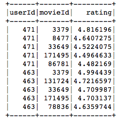
Lets go ahead and make recommendations based on our best model. recommendForAllUsers(n) function in als takes n recommedations. Lets go with 5 recommendations for all users.
让我们继续前进,并根据我们的最佳模型提出建议。 在als中的recommendedForAllUsers(n)函数需要n个建议。 让我们为所有用户提供5条建议。
# Generate n Recommendations for all users
recommendations = best_model.recommendForAllUsers(5)
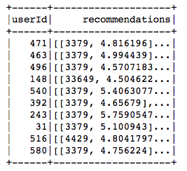
recommendations.show()
5.将建议转换为可解释的格式 (5. Convert recommendations into interpretable format)
The recommendations are generated in a format that easy to use in pyspark. As seen in the above the output, the recommendations are saved in an array format with movie id and ratings. To make these recommendations easy to read and compare t check if recommendations make sense, we will want to add more information like movie name and genre, then explode array to get rows with single recommendations.
推荐以易于在pyspark中使用的格式生成。 从上面的输出中可以看到,推荐以带有电影ID和等级的数组格式保存。 为了使这些建议易于阅读和比较,并检查建议是否有意义,我们将要添加更多信息,例如电影名称和流派,然后爆炸数组以获取包含单个建议的行。
nrecommendations = nrecommendations\
    .withColumn("rec_exp", explode("recommendations"))\
    .select('userId', col("rec_exp.movieId"), col("rec_exp.rating"))nrecommendations.limit(10).show()
这些建议有意义吗? (Do the recommendations make sense?)
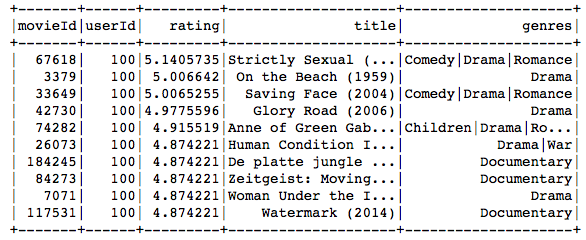
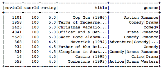
To check if the recommendations make sense, join movie name and genre to the above table. Lets randomly pick 100th user to check if the recommendations make sense.
要检查推荐的建议是否有意义,请将电影名称和类型加入上表。 让我们随机选择第100个用户来检查推荐是否有意义。
第100个用户的ALS建议: (100th User’s ALS Recommendations:)
nrecommendations.join(movies, on='movieId').filter('userId = 100').show()第100位使用者的实际偏好: (100th User’s Actual Preference:)
ratings.join(movies, on='movieId').filter('userId = 100').sort('rating', ascending=False).limit(10).show()The movie recommended to the 100th user primarily belongs to comedy, drama, war and romance genres, and the movies preferred by the user as seen in the above table, match very closely with these genres.
推荐给第100位用户的电影主要属于喜剧,戏剧,战争和浪漫类,而上表中用户偏爱的电影与这些流派非常匹配。
I hope you enjoyed reading. Please find the detailed codes in the Github Repository.
希望您喜欢阅读。 请在Github存储库中找到详细的代码。
翻译自: https://medium.com/swlh/build-recommendation-system-with-pyspark-using-alternating-least-squares-als-matrix-factorisation-ebe1ad2e7679
als pyspark
