pytroch、tensorflow对比学习—搭建模型范式（低阶、中阶、高阶API示例）

搭建模型范式（低阶、中阶、高阶API示例）

前言

本文是《pytorch-tensorflow-Comparative study》，pytorch和tensorflow对比学习专栏，第四章——搭建模型范式（低阶、中阶、高阶API示例）。

虽然说这两个框架在语法和接口的命名上有很多地方是不同的，但是深度学习的建模过程确实基本上都是一个套路的。

所以该笔记的笔记方式是：在使用相同的处理功能模块上，对比记录pytorch和tensorflow两者的API接口，和语法。

1，有利于深入理解深度学习建模过程流程。

2，有利于理解pytorch，和tensorflow设计上的不同，更加灵活的使用在自己的项目中。

3，有利于深入理解各个功能模块的使用。

本章节主要对比学习pytorch 和tensorflow有关搭建模型范式（低阶、中阶、高阶API示例）接口，和语法。

低阶API示例

这里范例使用Pytorch和tensorflow的低阶API分别实现线性回归模型和DNN二分类模型。

低阶API主要包括张量操作，计算图和自动微分。

先定义打印时间函数（在中介和高阶API示例中都会使用到）：

pytorch

import os
import datetime

#打印时间
def printbar():
    nowtime = datetime.datetime.now().strftime('%Y-%m-%d %H:%M:%S')
    print("\n"+"=========="*8 + "%s"%nowtime)

#mac系统上pytorch和matplotlib在jupyter中同时跑需要更改环境变量
os.environ["KMP_DUPLICATE_LIB_OK"]="TRUE" 

tensorflow

import tensorflow as tf

#打印时间分割线
@tf.function
def printbar():
    today_ts = tf.timestamp()%(24*60*60)

    hour = tf.cast(today_ts//3600+8,tf.int32)%tf.constant(24)
    minite = tf.cast((today_ts%3600)//60,tf.int32)
    second = tf.cast(tf.floor(today_ts%60),tf.int32)
    
    def timeformat(m):
        if tf.strings.length(tf.strings.format("{}",m))==1:
            return(tf.strings.format("0{}",m))
        else:
            return(tf.strings.format("{}",m))
    
    timestring = tf.strings.join([timeformat(hour),timeformat(minite),
                timeformat(second)],separator = ":")
    tf.print("=========="*8+timestring)

线性回归模型

准备数据

pytorch

import numpy as np 
import pandas as pd
from matplotlib import pyplot as plt 
import torch
from torch import nn


#样本数量
n = 400

# 生成测试用数据集
X = 10*torch.rand([n,2])-5.0  #torch.rand是均匀分布 
w0 = torch.tensor([[2.0],[-3.0]])
b0 = torch.tensor([[10.0]])
Y = X@w0 + b0 + torch.normal( 0.0,2.0,size = [n,1])  # @表示矩阵乘法,增加正态扰动

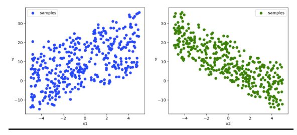
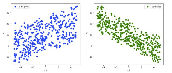
# 数据可视化
plt.figure(figsize = (12,5))
ax1 = plt.subplot(121)
ax1.scatter(X[:,0].numpy(),Y[:,0].numpy(), c = "b",label = "samples")
ax1.legend()
plt.xlabel("x1")
plt.ylabel("y",rotation = 0)

ax2 = plt.subplot(122)
ax2.scatter(X[:,1].numpy(),Y[:,0].numpy(), c = "g",label = "samples")
ax2.legend()
plt.xlabel("x2")
plt.ylabel("y",rotation = 0)
plt.show()

tensorflow

import numpy as np 
import pandas as pd
from matplotlib import pyplot as plt 
import tensorflow as tf


#样本数量
n = 400

# 生成测试用数据集
X = tf.random.uniform([n,2],minval=-10,maxval=10) 
w0 = tf.constant([[2.0],[-3.0]])
b0 = tf.constant([[3.0]])
Y = X@w0 + b0 + tf.random.normal([n,1],mean = 0.0,stddev= 2.0)  # @表示矩阵乘法,增加正态扰动

# 数据可视化
plt.figure(figsize = (12,5))
ax1 = plt.subplot(121)
ax1.scatter(X[:,0],Y[:,0], c = "b")
plt.xlabel("x1")
plt.ylabel("y",rotation = 0)

ax2 = plt.subplot(122)
ax2.scatter(X[:,1],Y[:,0], c = "g")
plt.xlabel("x2")
plt.ylabel("y",rotation = 0)
plt.show()

数据管道

pytroch

# 构建数据管道迭代器
def data_iter(features, labels, batch_size=8):
    num_examples = len(features)
    indices = list(range(num_examples))
    np.random.shuffle(indices)  #样本的读取顺序是随机的
    for i in range(0, num_examples, batch_size):
        indexs = torch.LongTensor(indices[i: min(i + batch_size, num_examples)])
        yield  features.index_select(0, indexs), labels.index_select(0, indexs)
        
# 测试数据管道效果   
batch_size = 8
(features,labels) = next(data_iter(X,Y,batch_size))
print(features)
print(labels)
# tensor([[-4.3880,  1.3655],
#         [-0.1082,  3.9533],
#         [-2.6286,  2.7058],
#         [ 1.0604, -1.8646],
#         [-1.5805,  1.5406],
#         [-2.6217, -3.2342],
#         [ 2.3748, -0.6449],
#         [-1.2478, -2.0509]])
# tensor([[-0.2069],
#         [-3.2494],
#         [-6.9620],
#         [17.0528],
#         [ 1.1076],
#         [17.2117],
#         [16.1081],
#         [14.7092]])

tensorflow

# 构建数据管道迭代器
def data_iter(features, labels, batch_size=8):
    num_examples = len(features)
    indices = list(range(num_examples))
    np.random.shuffle(indices)  #样本的读取顺序是随机的
    for i in range(0, num_examples, batch_size):
        indexs = indices[i: min(i + batch_size, num_examples)]
        yield tf.gather(features,indexs), tf.gather(labels,indexs)
        
# 测试数据管道效果   
batch_size = 8
(features,labels) = next(data_iter(X,Y,batch_size))
print(features)
print(labels)
# tf.Tensor(
# [[ 2.6161194   0.11071014]
#  [ 9.79207    -0.70180416]
#  [ 9.792343    6.9149055 ]
#  [-2.4186516  -9.375019  ]
#  [ 9.83749    -3.4637213 ]
#  [ 7.3953056   4.374569  ]
#  [-0.14686584 -0.28063297]
#  [ 0.49001217 -9.739792  ]], shape=(8, 2), dtype=float32)
# tf.Tensor(
# [[ 9.334667 ]
#  [22.058844 ]
#  [ 3.0695205]
#  [26.736238 ]
#  [35.292133 ]
#  [ 4.2943544]
#  [ 1.6713585]
#  [34.826904 ]], shape=(8, 1), dtype=float32)

定义模型

pytorch

# 定义模型
class LinearRegression: 
    
    def __init__(self):
        self.w = torch.randn_like(w0,requires_grad=True)
        self.b = torch.zeros_like(b0,requires_grad=True)
        
    #正向传播
    def forward(self,x): 
        return x@self.w + self.b

    # 损失函数
    def loss_func(self,y_pred,y_true):  
        return torch.mean((y_pred - y_true)**2/2)

model = LinearRegression()

tensorflow

w = tf.Variable(tf.random.normal(w0.shape))
b = tf.Variable(tf.zeros_like(b0,dtype = tf.float32))

# 定义模型
class LinearRegression:     
    #正向传播
    def __call__(self,x): 
        return x@w + b

    # 损失函数
    def loss_func(self,y_true,y_pred):  
        return tf.reduce_mean((y_true - y_pred)**2/2)

model = LinearRegression()

训练模型

def train_step(model, features, labels):
    
    predictions = model.forward(features)
    loss = model.loss_func(predictions,labels)
        
    # 反向传播求梯度
    loss.backward()
    
    # 使用torch.no_grad()避免梯度记录，也可以通过操作 model.w.data 实现避免梯度记录 
    with torch.no_grad():
        # 梯度下降法更新参数
        model.w -= 0.001*model.w.grad
        model.b -= 0.001*model.b.grad

        # 梯度清零
        model.w.grad.zero_()
        model.b.grad.zero_()
    return loss

# 测试train_step效果
batch_size = 10
(features,labels) = next(data_iter(X,Y,batch_size))
train_step(model,features,labels)
# tensor(92.8199, grad_fn=)

def train_model(model,epochs):
    for epoch in range(1,epochs+1):
        for features, labels in data_iter(X,Y,10):
            loss = train_step(model,features,labels)

        if epoch%200==0:
            printbar()
            print("epoch =",epoch,"loss = ",loss.item())
            print("model.w =",model.w.data)
            print("model.b =",model.b.data)

train_model(model,epochs = 1000)

# ================================================================================2020-07-05 08:27:57
# epoch = 200 loss =  2.6340413093566895
# model.w = tensor([[ 2.0283],
#         [-2.9632]])
# model.b = tensor([[10.0748]])
# 
# ================================================================================2020-07-05 08:28:00
# epoch = 400 loss =  2.24908709526062
# model.w = tensor([[ 2.0300],
#         [-2.9643]])
# model.b = tensor([[10.0781]])# 
# ....

tensorflow

'''
##使用autograph机制转换成静态图加速
@tf.function
'''
# 使用动态图调试
def train_step(model, features, labels):
    with tf.GradientTape() as tape:
        predictions = model(features)
        loss = model.loss_func(labels, predictions)
    # 反向传播求梯度
    dloss_dw,dloss_db = tape.gradient(loss,[w,b])
    # 梯度下降法更新参数
    w.assign(w - 0.001*dloss_dw)
    b.assign(b - 0.001*dloss_db)
    
    return loss

# 测试train_step效果
batch_size = 10
(features,labels) = next(data_iter(X,Y,batch_size))
train_step(model,features,labels)
# 

def train_model(model,epochs):
    for epoch in tf.range(1,epochs+1):
        for features, labels in data_iter(X,Y,10):
            loss = train_step(model,features,labels)

        if epoch%50==0:
            printbar()
            tf.print("epoch =",epoch,"loss = ",loss)
            tf.print("w =",w)
            tf.print("b =",b)

train_model(model,epochs = 200)

# ================================================================================16:35:56
# epoch = 50 loss =  1.78806472
# w = [[1.97554708]
#  [-2.97719598]]
# b = [[2.60692883]]
# ================================================================================16:36:00
# epoch = 100 loss =  2.64588404
# w = [[1.97319281]
#  [-2.97810626]]
# b = [[2.95525956]]
# ...

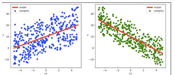
结果可视化

# 结果可视化

plt.figure(figsize = (12,5))
ax1 = plt.subplot(121)
ax1.scatter(X[:,0].numpy(),Y[:,0].numpy(), c = "b",label = "samples")
ax1.plot(X[:,0].numpy(),(model.w[0].data*X[:,0]+model.b[0].data).numpy(),"-r",linewidth = 5.0,label = "model")
ax1.legend()
plt.xlabel("x1")
plt.ylabel("y",rotation = 0)

ax2 = plt.subplot(122)
ax2.scatter(X[:,1].numpy(),Y[:,0].numpy(), c = "g",label = "samples")
ax2.plot(X[:,1].numpy(),(model.w[1].data*X[:,1]+model.b[0].data).numpy(),"-r",linewidth = 5.0,label = "model")
ax2.legend()
plt.xlabel("x2")
plt.ylabel("y",rotation = 0)

plt.show()

DNN二分类模型

准备数据

pytorch

import numpy as np 
import pandas as pd 
from matplotlib import pyplot as plt
import torch
from torch import nn
%matplotlib inline
%config InlineBackend.figure_format = 'svg'

#正负样本数量
n_positive,n_negative = 2000,2000

#生成正样本, 小圆环分布
r_p = 5.0 + torch.normal(0.0,1.0,size = [n_positive,1]) 
theta_p = 2*np.pi*torch.rand([n_positive,1])
Xp = torch.cat([r_p*torch.cos(theta_p),r_p*torch.sin(theta_p)],axis = 1)
Yp = torch.ones_like(r_p)

#生成负样本, 大圆环分布
r_n = 8.0 + torch.normal(0.0,1.0,size = [n_negative,1]) 
theta_n = 2*np.pi*torch.rand([n_negative,1])
Xn = torch.cat([r_n*torch.cos(theta_n),r_n*torch.sin(theta_n)],axis = 1)
Yn = torch.zeros_like(r_n)

#汇总样本
X = torch.cat([Xp,Xn],axis = 0)
Y = torch.cat([Yp,Yn],axis = 0)


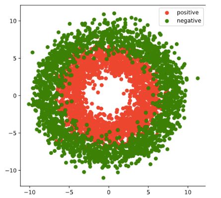
#可视化
plt.figure(figsize = (6,6))
plt.scatter(Xp[:,0].numpy(),Xp[:,1].numpy(),c = "r")
plt.scatter(Xn[:,0].numpy(),Xn[:,1].numpy(),c = "g")
plt.legend(["positive","negative"]);

tensorflow

import numpy as np 
import pandas as pd 
from matplotlib import pyplot as plt
import tensorflow as tf
%matplotlib inline
%config InlineBackend.figure_format = 'svg'

#正负样本数量
n_positive,n_negative = 2000,2000

#生成正样本, 小圆环分布
r_p = 5.0 + tf.random.truncated_normal([n_positive,1],0.0,1.0)
theta_p = tf.random.uniform([n_positive,1],0.0,2*np.pi) 
Xp = tf.concat([r_p*tf.cos(theta_p),r_p*tf.sin(theta_p)],axis = 1)
Yp = tf.ones_like(r_p)

#生成负样本, 大圆环分布
r_n = 8.0 + tf.random.truncated_normal([n_negative,1],0.0,1.0)
theta_n = tf.random.uniform([n_negative,1],0.0,2*np.pi) 
Xn = tf.concat([r_n*tf.cos(theta_n),r_n*tf.sin(theta_n)],axis = 1)
Yn = tf.zeros_like(r_n)

#汇总样本
X = tf.concat([Xp,Xn],axis = 0)
Y = tf.concat([Yp,Yn],axis = 0)


#可视化
plt.figure(figsize = (6,6))
plt.scatter(Xp[:,0].numpy(),Xp[:,1].numpy(),c = "r")
plt.scatter(Xn[:,0].numpy(),Xn[:,1].numpy(),c = "g")
plt.legend(["positive","negative"]);

数据管道

pytorch

# 构建数据管道迭代器
def data_iter(features, labels, batch_size=8):
    num_examples = len(features)
    indices = list(range(num_examples))
    np.random.shuffle(indices)  #样本的读取顺序是随机的
    for i in range(0, num_examples, batch_size):
        indexs = torch.LongTensor(indices[i: min(i + batch_size, num_examples)])
        yield  features.index_select(0, indexs), labels.index_select(0, indexs)
        
# 测试数据管道效果   
batch_size = 8
(features,labels) = next(data_iter(X,Y,batch_size))
print(features)
print(labels)
# tensor([[ 6.9914, -1.0820],
#         [ 4.8156,  4.0532],
#         [-1.0697, -7.4644],
#         [ 2.6291,  3.8851],
#         [-1.6780, -4.3390],
#         [-6.1495,  1.2269],
#         [-4.3422,  3.9552],
#         [-6.2265,  2.6159]])
# tensor([[0.],
#         [1.],
#         [0.],
#         [1.],
#         [1.],
#         [1.],
#         [1.],
#         [1.]])

tensorflow

# 构建数据管道迭代器
def data_iter(features, labels, batch_size=8):
    num_examples = len(features)
    indices = list(range(num_examples))
    np.random.shuffle(indices)  #样本的读取顺序是随机的
    for i in range(0, num_examples, batch_size):
        indexs = indices[i: min(i + batch_size, num_examples)]
        yield tf.gather(features,indexs), tf.gather(labels,indexs)
        
# 测试数据管道效果   
batch_size = 10
(features,labels) = next(data_iter(X,Y,batch_size))
print(features)
print(labels)
# tf.Tensor(
# [[ 0.03732629  3.5783494 ]
#  [ 0.542919    5.035079  ]
#  [ 5.860281   -2.4476354 ]
#  [ 0.63657564  3.194231  ]
#  [-3.5072308   2.5578873 ]
#  [-2.4109735  -3.6621518 ]
#  [ 4.0975413  -2.4172943 ]
#  [ 1.9393908  -6.782317  ]
#  [-4.7453732  -0.5176727 ]
#  [-1.4057113  -7.9775257 ]], shape=(10, 2), dtype=float32)
# tf.Tensor(
# [[1.]
#  [1.]
#  [0.]
#  [1.]
#  [1.]
#  [1.]
#  [1.]
#  [0.]
#  [1.]
#  [0.]], shape=(10, 1), dtype=float32)

定义模型

pythorch

此处范例我们利用nn.Module来组织模型变量。

class DNNModel(nn.Module):
    def __init__(self):
        super(DNNModel, self).__init__()
        self.w1 = nn.Parameter(torch.randn(2,4))
        self.b1 = nn.Parameter(torch.zeros(1,4))
        self.w2 = nn.Parameter(torch.randn(4,8))
        self.b2 = nn.Parameter(torch.zeros(1,8))
        self.w3 = nn.Parameter(torch.randn(8,1))
        self.b3 = nn.Parameter(torch.zeros(1,1))

    # 正向传播
    def forward(self,x):
        x = torch.relu(x@self.w1 + self.b1)
        x = torch.relu(x@self.w2 + self.b2)
        y = torch.sigmoid(x@self.w3 + self.b3)
        return y
    
    # 损失函数(二元交叉熵)
    def loss_func(self,y_pred,y_true):  
        #将预测值限制在1e-7以上, 1- (1e-7)以下，避免log(0)错误
        eps = 1e-7
        y_pred = torch.clamp(y_pred,eps,1.0-eps)
        bce = - y_true*torch.log(y_pred) - (1-y_true)*torch.log(1-y_pred)
        return torch.mean(bce)
    
    # 评估指标(准确率)
    def metric_func(self,y_pred,y_true):
        y_pred = torch.where(y_pred>0.5,torch.ones_like(y_pred,dtype = torch.float32),
                          torch.zeros_like(y_pred,dtype = torch.float32))
        acc = torch.mean(1-torch.abs(y_true-y_pred))
        return acc
    
model = DNNModel()

# 测试模型结构
batch_size = 10
(features,labels) = next(data_iter(X,Y,batch_size))

predictions = model(features)

loss = model.loss_func(labels,predictions)
metric = model.metric_func(labels,predictions)

print("init loss:", loss.item())
print("init metric:", metric.item())
# init loss: 7.979694366455078
# init metric: 0.50347900390625

len(list(model.parameters()))
# 6

tensorflow

此处范例我们利用tf.Module来组织模型变量，关于tf.Module的较详细介绍参考本书第四章最后一节: Autograph和tf.Module。

class DNNModel(tf.Module):
    def __init__(self,name = None):
        super(DNNModel, self).__init__(name=name)
        self.w1 = tf.Variable(tf.random.truncated_normal([2,4]),dtype = tf.float32)
        self.b1 = tf.Variable(tf.zeros([1,4]),dtype = tf.float32)
        self.w2 = tf.Variable(tf.random.truncated_normal([4,8]),dtype = tf.float32)
        self.b2 = tf.Variable(tf.zeros([1,8]),dtype = tf.float32)
        self.w3 = tf.Variable(tf.random.truncated_normal([8,1]),dtype = tf.float32)
        self.b3 = tf.Variable(tf.zeros([1,1]),dtype = tf.float32)

     
    # 正向传播
    @tf.function(input_signature=[tf.TensorSpec(shape = [None,2], dtype = tf.float32)])  
    def __call__(self,x):
        x = tf.nn.relu(x@self.w1 + self.b1)
        x = tf.nn.relu(x@self.w2 + self.b2)
        y = tf.nn.sigmoid(x@self.w3 + self.b3)
        return y
    
    # 损失函数(二元交叉熵)
    @tf.function(input_signature=[tf.TensorSpec(shape = [None,1], dtype = tf.float32),
                              tf.TensorSpec(shape = [None,1], dtype = tf.float32)])  
    def loss_func(self,y_true,y_pred):  
        #将预测值限制在 1e-7 以上, 1 - 1e-7 以下，避免log(0)错误
        eps = 1e-7
        y_pred = tf.clip_by_value(y_pred,eps,1.0-eps)
        bce = - y_true*tf.math.log(y_pred) - (1-y_true)*tf.math.log(1-y_pred)
        return  tf.reduce_mean(bce)
    
    # 评估指标(准确率)
    @tf.function(input_signature=[tf.TensorSpec(shape = [None,1], dtype = tf.float32),
                              tf.TensorSpec(shape = [None,1], dtype = tf.float32)]) 
    def metric_func(self,y_true,y_pred):
        y_pred = tf.where(y_pred>0.5,tf.ones_like(y_pred,dtype = tf.float32),
                          tf.zeros_like(y_pred,dtype = tf.float32))
        acc = tf.reduce_mean(1-tf.abs(y_true-y_pred))
        return acc
    
model = DNNModel()

# 测试模型结构
batch_size = 10
(features,labels) = next(data_iter(X,Y,batch_size))

predictions = model(features)

loss = model.loss_func(labels,predictions)
metric = model.metric_func(labels,predictions)

tf.print("init loss:",loss)
tf.print("init metric",metric)
# init loss: 1.76568353
# init metric 0.6
print(len(model.trainable_variables))
# 6

训练模型

pytorch

def train_step(model, features, labels):   
    
    # 正向传播求损失
    predictions = model.forward(features)
    loss = model.loss_func(predictions,labels)
    metric = model.metric_func(predictions,labels)
        
    # 反向传播求梯度
    loss.backward()
    
    # 梯度下降法更新参数
    for param in model.parameters():
        #注意是对param.data进行重新赋值,避免此处操作引起梯度记录
        param.data = (param.data - 0.01*param.grad.data) 
        
    # 梯度清零
    model.zero_grad()
        
    return loss.item(),metric.item()
 

def train_model(model,epochs):
    for epoch in range(1,epochs+1):
        loss_list,metric_list = [],[]
        for features, labels in data_iter(X,Y,20):
            lossi,metrici = train_step(model,features,labels)
            loss_list.append(lossi)
            metric_list.append(metrici)
        loss = np.mean(loss_list)
        metric = np.mean(metric_list)

        if epoch%100==0:
            printbar()
            print("epoch =",epoch,"loss = ",loss,"metric = ",metric)
        
train_model(model,epochs = 1000)
# ================================================================================2020-07-05 08:32:16
# epoch = 100 loss =  0.24841043589636683 metric =  0.8944999960064888
# 
# ================================================================================2020-07-05 08:32:34
# epoch = 200 loss =  0.20398724960163236 metric =  0.920999992787838
# 
# ================================================================================2020-07-05 08:32:54
# epoch = 300 loss =  0.19509393003769218 metric =  0.9239999914169311
# 
# ================================================================================2020-07-05 08:33:14
# ...

tensorflow

##使用autograph机制转换成静态图加速

@tf.function
def train_step(model, features, labels):
    
    # 正向传播求损失
    with tf.GradientTape() as tape:
        predictions = model(features)
        loss = model.loss_func(labels, predictions) 
        
    # 反向传播求梯度
    grads = tape.gradient(loss, model.trainable_variables)
    
    # 执行梯度下降
    for p, dloss_dp in zip(model.trainable_variables,grads):
        p.assign(p - 0.001*dloss_dp)
        
    # 计算评估指标
    metric = model.metric_func(labels,predictions)
    
    return loss, metric


def train_model(model,epochs):
    for epoch in tf.range(1,epochs+1):
        for features, labels in data_iter(X,Y,100):
            loss,metric = train_step(model,features,labels)
        if epoch%100==0:
            printbar()
            tf.print("epoch =",epoch,"loss = ",loss, "accuracy = ", metric)
        

train_model(model,epochs = 600)

# ================================================================================16:47:35
# epoch = 100 loss =  0.567795336 accuracy =  0.71
# ================================================================================16:47:39
# epoch = 200 loss =  0.50955683 accuracy =  0.77
# ================================================================================16:47:43
# epoch = 300 loss =  0.421476126 accuracy =  0.84

结果可视化

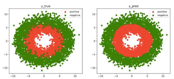
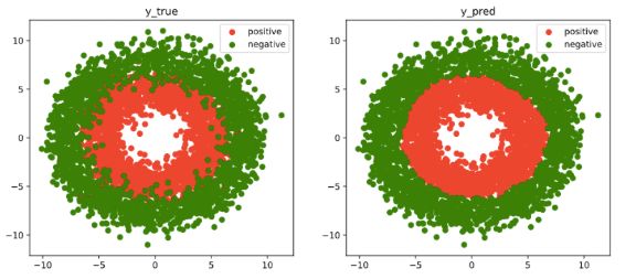
fig, (ax1,ax2) = plt.subplots(nrows=1,ncols=2,figsize = (12,5))
ax1.scatter(Xp[:,0],Xp[:,1], c="r")
ax1.scatter(Xn[:,0],Xn[:,1],c = "g")
ax1.legend(["positive","negative"]);
ax1.set_title("y_true");

Xp_pred = X[torch.squeeze(model.forward(X)>=0.5)]
Xn_pred = X[torch.squeeze(model.forward(X)<0.5)]

ax2.scatter(Xp_pred[:,0],Xp_pred[:,1],c = "r")
ax2.scatter(Xn_pred[:,0],Xn_pred[:,1],c = "g")
ax2.legend(["positive","negative"]);
ax2.set_title("y_pred");

中介API示例

Pytorch的中阶API主要包括各种模型层，损失函数，优化器，数据管道等等。

TensorFlow的中阶API主要包括各种模型层，损失函数，优化器，数据管道，特征列等等。

线性回归模型

准备数据

pytroch和tensorflow 的数据准备和低阶API部分相同，使用相同的数据，可以直接把代码粘过来，这里不做重复。

数据管道

pytroch

#构建输入数据管道
ds = TensorDataset(X,Y)
dl = DataLoader(ds,batch_size = 10,shuffle=True,num_workers=2)

tensorflow

#构建输入数据管道
ds = tf.data.Dataset.from_tensor_slices((X,Y)) \
     .shuffle(buffer_size = 100).batch(10) \
     .prefetch(tf.data.experimental.AUTOTUNE)  

定义模型

pytroch

model = nn.Linear(2,1) #线性层

model.loss_func = nn.MSELoss()
model.optimizer = torch.optim.SGD(model.parameters(),lr = 0.01)

tensorflow

model = layers.Dense(units = 1) 
model.build(input_shape = (2,)) #用build方法创建variables
model.loss_func = losses.mean_squared_error
model.optimizer = optimizers.SGD(learning_rate=0.001)

训练模型

pytorch

def train_step(model, features, labels):
    
    predictions = model(features)
    loss = model.loss_func(predictions,labels)
    loss.backward()
    model.optimizer.step()
    model.optimizer.zero_grad()
    return loss.item()

# 测试train_step效果
features,labels = next(iter(dl))
train_step(model,features,labels)
# 269.98016357421875

def train_model(model,epochs):
    for epoch in range(1,epochs+1):
        for features, labels in dl:
            loss = train_step(model,features,labels)
        if epoch%50==0:
            printbar()
            w = model.state_dict()["weight"]
            b = model.state_dict()["bias"]
            print("epoch =",epoch,"loss = ",loss)
            print("w =",w)
            print("b =",b)
train_model(model,epochs = 200)

# ================================================================================2020-07-05 22:51:53
# epoch = 50 loss =  3.0177409648895264
# w = tensor([[ 1.9315, -2.9573]])
# b = tensor([9.9625])
# 
# ================================================================================2020-07-05 22:51:57
# epoch = 100 loss =  2.1144354343414307
# w = tensor([[ 1.9760, -2.9398]])
# b = tensor([9.9428])
# ...

tensorflow

#使用autograph机制转换成静态图加速

@tf.function
def train_step(model, features, labels):
    with tf.GradientTape() as tape:
        predictions = model(features)
        loss = model.loss_func(tf.reshape(labels,[-1]), tf.reshape(predictions,[-1]))
    grads = tape.gradient(loss,model.variables)
    model.optimizer.apply_gradients(zip(grads,model.variables))
    return loss

# 测试train_step效果
features,labels = next(ds.as_numpy_iterator())
train_step(model,features,labels)

def train_model(model,epochs):
    for epoch in tf.range(1,epochs+1):
        loss = tf.constant(0.0)
        for features, labels in ds:
            loss = train_step(model,features,labels)
        if epoch%50==0:
            printbar()
            tf.print("epoch =",epoch,"loss = ",loss)
            tf.print("w =",model.variables[0])
            tf.print("b =",model.variables[1])
train_model(model,epochs = 200)
# ===========================================================================17:01:48
# epoch = 50 loss =  2.56481647
# w = [[1.99355531]
#  [-2.99061537]]
# b = [3.09484935]
# ===========================================================================17:01:51
# epoch = 100 loss =  5.96198225
# w = [[1.98028314]
#  [-2.96975136]]
# b = [3.09501529]
# ...

结果可视化

代码同上章节

DNN二分类模型

准备数据

pytroch和tensorflow 的数据准备和低阶API部分相同，使用相同的数据，可以直接把代码粘过来，这里不做重复。

数据管道

pytorch

#构建输入数据管道
ds = TensorDataset(X,Y)
dl = DataLoader(ds,batch_size = 10,shuffle=True,num_workers=2)

tensorflow

#构建输入数据管道
ds = tf.data.Dataset.from_tensor_slices((X,Y)) \
     .shuffle(buffer_size = 4000).batch(100) \
     .prefetch(tf.data.experimental.AUTOTUNE) 

定义模型

pytroch

class DNNModel(nn.Module):
    def __init__(self):
        super(DNNModel, self).__init__()
        self.fc1 = nn.Linear(2,4)
        self.fc2 = nn.Linear(4,8) 
        self.fc3 = nn.Linear(8,1)

    # 正向传播
    def forward(self,x):
        x = F.relu(self.fc1(x))
        x = F.relu(self.fc2(x))
        y = nn.Sigmoid()(self.fc3(x))
        return y
    
    # 损失函数
    def loss_func(self,y_pred,y_true):
        return nn.BCELoss()(y_pred,y_true)
    
    # 评估函数(准确率)
    def metric_func(self,y_pred,y_true):
        y_pred = torch.where(y_pred>0.5,torch.ones_like(y_pred,dtype = torch.float32),
                          torch.zeros_like(y_pred,dtype = torch.float32))
        acc = torch.mean(1-torch.abs(y_true-y_pred))
        return acc
    
    # 优化器
    @property
    def optimizer(self):
        return torch.optim.Adam(self.parameters(),lr = 0.001)
    
model = DNNModel()

# 测试模型结构
(features,labels) = next(iter(dl))
predictions = model(features)

loss = model.loss_func(predictions,labels)
metric = model.metric_func(predictions,labels)

print("init loss:",loss.item())
print("init metric:",metric.item())
# init loss: 0.7065666913986206
# init metric: 0.6000000238418579

tensorflow

class DNNModel(tf.Module):
    def __init__(self,name = None):
        super(DNNModel, self).__init__(name=name)
        self.dense1 = layers.Dense(4,activation = "relu") 
        self.dense2 = layers.Dense(8,activation = "relu")
        self.dense3 = layers.Dense(1,activation = "sigmoid")

     
    # 正向传播
    @tf.function(input_signature=[tf.TensorSpec(shape = [None,2], dtype = tf.float32)])  
    def __call__(self,x):
        x = self.dense1(x)
        x = self.dense2(x)
        y = self.dense3(x)
        return y
    
model = DNNModel()
model.loss_func = losses.binary_crossentropy
model.metric_func = metrics.binary_accuracy
model.optimizer = optimizers.Adam(learning_rate=0.001)

# 测试模型结构
(features,labels) = next(ds.as_numpy_iterator())

predictions = model(features)

loss = model.loss_func(tf.reshape(labels,[-1]),tf.reshape(predictions,[-1]))
metric = model.metric_func(tf.reshape(labels,[-1]),tf.reshape(predictions,[-1]))

tf.print("init loss:",loss)
tf.print("init metric",metric)
# init loss: 1.13653195
# init metric 0.5

训练模型

pytroch

def train_step(model, features, labels):
    
    # 正向传播求损失
    predictions = model(features)
    loss = model.loss_func(predictions,labels)
    metric = model.metric_func(predictions,labels)
    
    # 反向传播求梯度
    loss.backward()
    
    # 更新模型参数
    model.optimizer.step()
    model.optimizer.zero_grad()
    
    return loss.item(),metric.item()

# 测试train_step效果
features,labels = next(iter(dl))
train_step(model,features,labels)
# (0.6048880815505981, 0.699999988079071)

def train_model(model,epochs):
    for epoch in range(1,epochs+1):
        loss_list,metric_list = [],[]
        for features, labels in dl:
            lossi,metrici = train_step(model,features,labels)
            loss_list.append(lossi)
            metric_list.append(metrici)
        loss = np.mean(loss_list)
        metric = np.mean(metric_list)

        if epoch%100==0:
            printbar()
            print("epoch =",epoch,"loss = ",loss,"metric = ",metric)
        
train_model(model,epochs = 300)
# ==============================================================2020-07-05 22:56:38
# epoch = 100 loss =  0.23532892110607917 metric =  0.934749992787838
# 
# ==============================================================2020-07-05 22:58:18
# epoch = 200 loss =  0.24743918558603128 metric =  0.934999993443489

tensorflow

#使用autograph机制转换成静态图加速

@tf.function
def train_step(model, features, labels):
    with tf.GradientTape() as tape:
        predictions = model(features)
        loss = model.loss_func(tf.reshape(labels,[-1]), tf.reshape(predictions,[-1]))
    grads = tape.gradient(loss,model.trainable_variables)
    model.optimizer.apply_gradients(zip(grads,model.trainable_variables))
    
    metric = model.metric_func(tf.reshape(labels,[-1]), tf.reshape(predictions,[-1]))
    
    return loss,metric

# 测试train_step效果
features,labels = next(ds.as_numpy_iterator())
train_step(model,features,labels)
# (,
#  )

def train_model(model,epochs):
    for epoch in tf.range(1,epochs+1):
        loss, metric = tf.constant(0.0),tf.constant(0.0)
        for features, labels in ds:
            loss,metric = train_step(model,features,labels)
        if epoch%10==0:
            printbar()
            tf.print("epoch =",epoch,"loss = ",loss, "accuracy = ",metric)
train_model(model,epochs = 60)

# ========================================================================17:07:36
# epoch = 10 loss =  0.556449413 accuracy =  0.79
# ========================================================================17:07:38
# epoch = 20 loss =  0.439187407 accuracy =  0.86
# ...

结果可视化

代码同上章节

高阶API示例

TensorFlow的高阶API主要为tf.keras.models提供的模型的类接口。

使用Keras接口有以下3种方式构建模型：使用Sequential按层顺序构建模型，使用函数式API构建任意结构模型，继承Model基类构建自定义模型。

此处分别演示使用Sequential按层顺序构建模型以及继承Model基类构建自定义模型。

Pytorch没有官方的高阶API，一般需要用户自己实现训练循环、验证循环、和预测循环。

不过有大神通过仿照tf.keras.Model的功能对Pytorch的nn.Module进行了封装，设计了torchkeras.Model类，

实现了 fit, validate，predict, summary 方法，相当于用户自定义高阶API。

并示范了用它实现线性回归模型。

此外，还通过借用pytorch_lightning的功能，封装了类Keras接口的另外一种实现，即torchkeras.LightModel类。

pytorch

此范例我们通过继承torchkeras.Model模型接口，实现线性回归模型。

tensorflow

此范例我们使用Sequential按层顺序构建模型，并使用内置model.fit方法训练模型【面向新手】。

线性回归模型

准备数据

代码同上章节

数据管道

pytroch

#构建输入数据管道
ds = TensorDataset(X,Y)
ds_train,ds_valid = torch.utils.data.random_split(ds,[int(400*0.7),400-int(400*0.7)])
dl_train = DataLoader(ds_train,batch_size = 10,shuffle=True,num_workers=2)
dl_valid = DataLoader(ds_valid,batch_size = 10,num_workers=2)

tensorflow

数据管道的构建继承在高阶API训练阶段的参数上

定义模型

pytorch

# 继承用户自定义模型
from torchkeras import Model
class LinearRegression(Model):
    def __init__(self):
        super(LinearRegression, self).__init__()
        self.fc = nn.Linear(2,1)
    
    def forward(self,x):
        return self.fc(x)

model = LinearRegression()

model.summary(input_shape = (2,))
"""
----------------------------------------------------------------
        Layer (type)               Output Shape         Param #
================================================================
            Linear-1                    [-1, 1]               3
================================================================
Total params: 3
Trainable params: 3
Non-trainable params: 0
----------------------------------------------------------------
Input size (MB): 0.000008
Forward/backward pass size (MB): 0.000008
Params size (MB): 0.000011
Estimated Total Size (MB): 0.000027
----------------------------------------------------------------
"""

tensorflow

tf.keras.backend.clear_session()

model = models.Sequential()
model.add(layers.Dense(1,input_shape =(2,)))
model.summary()

""""
Model: "sequential"
_________________________________________________________________
Layer (type)                 Output Shape              Param #   
=================================================================
dense (Dense)                (None, 1)                 3         
=================================================================
Total params: 3
Trainable params: 3
Non-trainable params: 0
"""

训练模型

pytroch

### 使用fit方法进行训练

def mean_absolute_error(y_pred,y_true):
    return torch.mean(torch.abs(y_pred-y_true))

def mean_absolute_percent_error(y_pred,y_true):
    absolute_percent_error = (torch.abs(y_pred-y_true)+1e-7)/(torch.abs(y_true)+1e-7)
    return torch.mean(absolute_percent_error)

model.compile(loss_func = nn.MSELoss(),
              optimizer= torch.optim.Adam(model.parameters(),lr = 0.01),
              metrics_dict={"mae":mean_absolute_error,"mape":mean_absolute_percent_error})

dfhistory = model.fit(200,dl_train = dl_train, dl_val = dl_valid,log_step_freq = 20)

"""
Start Training ...

================================================================================2020-07-05 23:07:25
{'step': 20, 'loss': 226.768, 'mae': 12.198, 'mape': 1.212}

 +-------+---------+-------+-------+----------+---------+----------+
| epoch |   loss  |  mae  |  mape | val_loss | val_mae | val_mape |
+-------+---------+-------+-------+----------+---------+----------+
|   1   | 230.773 | 12.41 | 1.394 | 223.262  |  12.582 |  1.095   |
+-------+---------+-------+-------+----------+---------+----------+

================================================================================2020-07-05 23:07:26
{'step': 20, 'loss': 200.964, 'mae': 11.584, 'mape': 1.382}

 +-------+---------+--------+------+----------+---------+----------+
| epoch |   loss  |  mae   | mape | val_loss | val_mae | val_mape |
+-------+---------+--------+------+----------+---------+----------+
|   2   | 206.238 | 11.759 | 1.26 | 199.669  |  11.895 |  1.012   |
+-------+---------+--------+------+----------+---------+----------+
...
“”“

tensorflow

### 使用fit方法进行训练

model.compile(optimizer="adam",loss="mse",metrics=["mae"])
model.fit(X,Y,batch_size = 10,epochs = 200)  

tf.print("w = ",model.layers[0].kernel)
tf.print("b = ",model.layers[0].bias)

Epoch 197/200
400/400 [==============================] - 0s 190us/sample - loss: 4.3977 - mae: 1.7129
Epoch 198/200
400/400 [==============================] - 0s 172us/sample - loss: 4.3918 - mae: 1.7117
Epoch 199/200
400/400 [==============================] - 0s 134us/sample - loss: 4.3861 - mae: 1.7106
Epoch 200/200
400/400 [==============================] - 0s 166us/sample - loss: 4.3786 - mae: 1.7092
w =  [[1.99339032]
 [-3.00866461]]
b =  [2.67018795]

结果可视化

DNN二分类模型

pytorch中：此范例我们通过继承torchkeras.LightModel模型接口，实现DNN二分类模型。

**tensorflow中：**此范例我们使用继承Model基类构建自定义模型，并构建自定义训练循环【面向专家】

准备数据

代码同上章节

数据管道

pytorch

ds = TensorDataset(X,Y)

ds_train,ds_valid = torch.utils.data.random_split(ds,[int(len(ds)*0.7),len(ds)-int(len(ds)*0.7)])
dl_train = DataLoader(ds_train,batch_size = 100,shuffle=True,num_workers=2)
dl_valid = DataLoader(ds_valid,batch_size = 100,num_workers=2)

tensorflow

ds_train = tf.data.Dataset.from_tensor_slices((X[0:n*3//4,:],Y[0:n*3//4,:])) \
     .shuffle(buffer_size = 1000).batch(20) \
     .prefetch(tf.data.experimental.AUTOTUNE) \
     .cache()

ds_valid = tf.data.Dataset.from_tensor_slices((X[n*3//4:,:],Y[n*3//4:,:])) \
     .batch(20) \
     .prefetch(tf.data.experimental.AUTOTUNE) \
     .cache()

定义模型

pytorch

class Net(nn.Module):
    def __init__(self):
        super().__init__()
        self.fc1 = nn.Linear(2,4)
        self.fc2 = nn.Linear(4,8) 
        self.fc3 = nn.Linear(8,1)
        
    def forward(self,x):
        x = F.relu(self.fc1(x))
        x = F.relu(self.fc2(x))
        y = nn.Sigmoid()(self.fc3(x))
        return y
        
class Model(torchkeras.LightModel):
    
    #loss,and optional metrics
    def shared_step(self,batch)->dict:
        x, y = batch
        prediction = self(x)
        loss = nn.BCELoss()(prediction,y)
        preds = torch.where(prediction>0.5,torch.ones_like(prediction),torch.zeros_like(prediction))
        acc = pl.metrics.functional.accuracy(preds, y)
        # attention: there must be a key of "loss" in the returned dict 
        dic = {"loss":loss,"acc":acc} 
        return dic
    
    #optimizer,and optional lr_scheduler
    def configure_optimizers(self):
        optimizer = torch.optim.Adam(self.parameters(), lr=1e-2)
        lr_scheduler = torch.optim.lr_scheduler.StepLR(optimizer, step_size=10, gamma=0.0001)
        return {"optimizer":optimizer,"lr_scheduler":lr_scheduler}
    
pl.seed_everything(1234)
net = Net()
model = Model(net)


torchkeras.summary(model,input_shape =(2,))

----------------------------------------------------------------
        Layer (type)               Output Shape         Param #
================================================================
            Linear-1                    [-1, 4]              12
            Linear-2                    [-1, 8]              40
            Linear-3                    [-1, 1]               9
================================================================
Total params: 61
Trainable params: 61
Non-trainable params: 0
----------------------------------------------------------------
Input size (MB): 0.000008
Forward/backward pass size (MB): 0.000099
Params size (MB): 0.000233
Estimated Total Size (MB): 0.000340
----------------------------------------------------------------

tensorflow

tf.keras.backend.clear_session()
class DNNModel(models.Model):
    def __init__(self):
        super(DNNModel, self).__init__()
        
    def build(self,input_shape):
        self.dense1 = layers.Dense(4,activation = "relu",name = "dense1") 
        self.dense2 = layers.Dense(8,activation = "relu",name = "dense2")
        self.dense3 = layers.Dense(1,activation = "sigmoid",name = "dense3")
        super(DNNModel,self).build(input_shape)
 
    # 正向传播
    @tf.function(input_signature=[tf.TensorSpec(shape = [None,2], dtype = tf.float32)])  
    def call(self,x):
        x = self.dense1(x)
        x = self.dense2(x)
        y = self.dense3(x)
        return y

model = DNNModel()
model.build(input_shape =(None,2))

model.summary()

Model: "dnn_model"
_________________________________________________________________
Layer (type)                 Output Shape              Param #   
=================================================================
dense1 (Dense)               multiple                  12        
_________________________________________________________________
dense2 (Dense)               multiple                  40        
_________________________________________________________________
dense3 (Dense)               multiple                  9         
=================================================================
Total params: 61
Trainable params: 61
Non-trainable params: 0
_________________________________________________________________

训练模型

pytroch

ckpt_cb = pl.callbacks.ModelCheckpoint(monitor='val_loss')

# set gpus=0 will use cpu，
# set gpus=1 will use 1 gpu
# set gpus=2 will use 2gpus 
# set gpus = -1 will use all gpus 
# you can also set gpus = [0,1] to use the  given gpus
# you can even set tpu_cores=2 to use two tpus 

trainer = pl.Trainer(max_epochs=100,gpus = 0, callbacks=[ckpt_cb]) 

trainer.fit(model,dl_train,dl_valid)

=============================================================2021-01-16 23:41:38
epoch =  0
{'val_loss': 0.6706896424293518, 'val_acc': 0.5558333396911621}
{'acc': 0.5157142281532288, 'loss': 0.6820458769798279}

============================================================2021-01-16 23:41:39
epoch =  1
{'val_loss': 0.653035581111908, 'val_acc': 0.5708333849906921}
{'acc': 0.5457143783569336, 'loss': 0.6677185297012329}
...

tensorflow

### 自定义训练循环

optimizer = optimizers.Adam(learning_rate=0.01)
loss_func = tf.keras.losses.BinaryCrossentropy()

train_loss = tf.keras.metrics.Mean(name='train_loss')
train_metric = tf.keras.metrics.BinaryAccuracy(name='train_accuracy')

valid_loss = tf.keras.metrics.Mean(name='valid_loss')
valid_metric = tf.keras.metrics.BinaryAccuracy(name='valid_accuracy')


@tf.function
def train_step(model, features, labels):
    with tf.GradientTape() as tape:
        predictions = model(features)
        loss = loss_func(labels, predictions)
    grads = tape.gradient(loss, model.trainable_variables)
    optimizer.apply_gradients(zip(grads, model.trainable_variables))

    train_loss.update_state(loss)
    train_metric.update_state(labels, predictions)

@tf.function
def valid_step(model, features, labels):
    predictions = model(features)
    batch_loss = loss_func(labels, predictions)
    valid_loss.update_state(batch_loss)
    valid_metric.update_state(labels, predictions)
    

def train_model(model,ds_train,ds_valid,epochs):
    for epoch in tf.range(1,epochs+1):
        for features, labels in ds_train:
            train_step(model,features,labels)

        for features, labels in ds_valid:
            valid_step(model,features,labels)

        logs = 'Epoch={},Loss:{},Accuracy:{},Valid Loss:{},Valid Accuracy:{}'
        
        if  epoch%100 ==0:
            printbar()
            tf.print(tf.strings.format(logs,
            (epoch,train_loss.result(),train_metric.result(),valid_loss.result(),valid_metric.result())))
        
        train_loss.reset_states()
        valid_loss.reset_states()
        train_metric.reset_states()
        valid_metric.reset_states()

train_model(model,ds_train,ds_valid,1000)

================================================================================17:35:02
Epoch=100,Loss:0.194088802,Accuracy:0.923064,Valid Loss:0.215538561,Valid Accuracy:0.904368
================================================================================17:35:22
Epoch=200,Loss:0.151239693,Accuracy:0.93768847,Valid Loss:0.181166962,Valid Accuracy:0.920664132
================================================================================17:35:43
Epoch=300,Loss:0.134556711,Accuracy:0.944247484,Valid Loss:0.171530813,Valid Accuracy:0.926396072

结果可视化

代码同上章节

说明

笔记中很多代码案例来自于：

《20天吃掉那只Pytorch》

• github项目地址: https://github.com/lyhue1991/eat_pytorch_in_20_days

《30天吃掉那只TensorFlow2》

• github项目地址: https://github.com/lyhue1991/eat_tensorflow2_in_30_days

感兴趣的同学可以进入学习。

===========================================================================

我的笔记一部分是将这两项目中内容整理归纳，一部分是相应功能的内容自己找资料整理归纳。

笔记以MD格式存入我的git仓库，另外代码案例所需要数据集文件也在其中：可以clone下来学习使用。

《pytorch-tensorflow对比学习笔记》

github项目地址: https://github.com/Boris-2021/pytorch-tensorflow-Comparative-study

===========================================================================

笔记中增加了很多趣味性的图片，增加阅读乐趣。

===========================================================================

感觉对你的学习有帮助，就点个星，点个赞，点个关注再走把，整理不易，拒绝白嫖从我做起！