模板匹配--Image Alignment Algorithms - Part II

Implementing and comparing the forwards compositional and the Hager-Belhumeur algorithms.

• Download demo - 90 KB
• Download experiments - 71.9 KB

Introduction

Image alignment is an iterative minimization process of matching two images, template T and another image I. During the last 20 years, an image alignment technique proposed by Lucas and Kanade in 1981 has been widely used in computer vision. This technique uses image intensity gradient information to iteratively search for the best match between two images.

In the Lucas-Kanade 20 Years On: A Unifying Framework series of articles, S. Baker and I. Matthews describe and provide an implementation in Matlab of the following image alignment algorithms based on the Lucas-Kanade technique:

1. Forwards additive algorithm (the original Lucas-Kanade algorithm);
2. Forwards compositional algorithm;
3. Inverse compositional algorithm (proposed by Baker, Dellaert, and Matthews);
4. Inverse additive algorithm (proposed by Hager and Belhumeur).

Each image alignment algorithm iteratively minimizes the sum of square differences between the template T and image I, . Here, E(p) is the image similarity function, p is the vector of warp parameters, x is the pixel coordinates vector, I(x) and T(x) are intensity values of the pixel x of image I and image T, respectively.

In Image Alignment Algorithms – Part I, we described the first and the third of the algorithms mentioned above. In this article, we implement the other two algorithms, the inverse additive algorithm and the forwards compositional algorithm. We also modify the code of the first and the third algorithms to make them all comparable, and finally, we show which one is better (by meaning of speed and convergence) and decide if a real-time object tracking system can be built based on any of them.

Compiling example code

To experiment with the code, you need to compile it yourself. First of all, you need Visual Studio to be installed. Visual C++ Express Edition also fits our needs.

Then, you need to download and install the OpenCV library from here. OpenCV is an Intel open source computer vision library, and we will use it as the base for our code. Download OpenCV_1.0.exe and run its installer on your computer.

And at last, you need to configure your Visual Studio as follows. In the Visual Studio main window, choose the Tools -> Options... menu item, then click the Projects and Solutions -> VC++ Directories tree item.

In the 'Show directories for..' combo box, select 'Library Files'. Add the following line to the list below:

Hide    Copy Code

C:\Program Files\OpenCV\lib

In the 'Show directories for..' combo box, select 'Include Files'. Add the following lines to the list below:

Hide    Copy Code

C:\Program Files\OpenCV\cv\include
C:\Program Files\OpenCV\cxcore\include
C:\Program Files\OpenCV\otherlibs\highgui

That's all! Now, you can compile and run the project.

Structure of the project

The align_demo project contains the following files:

Files	Their content
auxfunc.h, auxfunc.cpp	Contains image warping functions.
forwadditive.h, forwadditive.cpp	Contains implementation of the Lucas-Kanade (forwards additive) algorithm.
forwcomp.h, forwcomp.cpp	Contains implementation of the forwards compositional algorithm.
invadditive.h, invadditive.cpp	Contains implementation of the Hager-Belhumeur (inverse additive) algorithm.
invcomp.h, invcomp.cpp	Contains implementation of the Baker-Dellaert-Matthews (inverse compositional) algorithm.

What does it do?

When you run the align_demo.exe, you can see a console window. You need to enter the image deformation parameters (components of the parameter vector p) and press Enter.

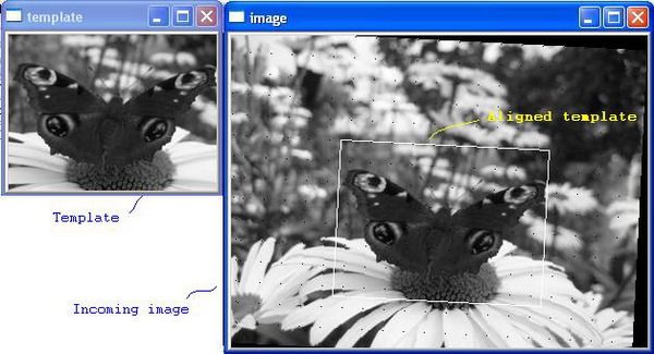
After that, you can see two windows, named «template» and «image». And, you can see the white rectangle denoting the initial approximation of the template T.

Then, you will be asked to press any key to run the Lucas-Kanade algorithm. Please ensure that the «image» or the «template» window has focus, otherwise the key press will have no effect.

When the Lucas-Kanade algorithm finishes, you can see the summary information, including the calculation time, the iteration count, and the resulting mean error. The resulting mean error  shows the quality of the alignment. The white rectangle in the «image» window displays the resulting template position approximation. Also, the log file is created. Each line of the log file contains the iteration number and the mean error on that iteration. You can find the log file (forwadditive.txt) in the align_demo folder. We will use the log files created for each algorithm to create graphs and compare the speed of convergence.

After that, you will be asked to press any key to run the Hager-Belhumeur algorithm, and so on. For each algorithm, the summary is displayed and the log file is created.

Finally, press any key to exit the application.

Implementing the Hager-Belhumeur (inverse additive) algorithm

We start with the Hager-Belhumeur algorithm (you can find its original description here), because it is a rather specific method. Its authors try to achieve computational efficiency of the method, that's why they require that the warp W has a specific form. The requirement is that the product of two Jacobians can be written as, , where  is a matrix that is just a function of the template coordinates, and is just a function of the warp parameters.

The warp matrix  that we used in Part I of this article doesn't have such a form. So we need to take another warp. Let's take this one: . This warp can model in-plane rotation, translation, and scaling of the template.

The warp parameter vector has the form of , where  is the rotation parameter,  and are translation parameters, and s is the scale parameter.

The coordinates of a warped pixel are calculated as the product of the warp matrix W(p) and the coordinate vector :

So, the Jacobians are calculated as follows: ; . The inverse of the last one is calculated as: .

After some algebraic manipulations, the product of these two Jacobians can be written in the required form of: .

Another requirement is that  must be invertible. The inverse of our Jacobian  is .

Hager-Belhumeur algorithm:

Pre-compute:

1. Evaluate the gradient  of the template T(x).
2. Evaluate .
3. Compute the modified steepest descent images: .
4. Compute the modified Hessian: .

Iterate:

5. Warp I with W(x;p) to compute I(W(x;p)).
6. Compute the error image I(W(x;p))-T(x).
7. Compute .
8. Compute .
9. Compute  and update .

until .

The Hager-Belhumeur algorithm is implemented in invadditive.h and invadditive.cpp.

Parameters for the algorithm are the template image T, the rectangular region of the template (let's denote it as omega), and the image I.

Hide    Copy Code

// Hager-Belhumeur inverse additive method
// @param[in] pImgT   Template image T
// @param[in] omega   Rectangular template region
// @param[in] pImgI   Another image I

void align_image_inverse_additive(IplImage* pImgT, CvRect omega, IplImage* pImgI)
{
    // Some constants for iterative minimization process.
    const float EPS = 1E-5f; // Threshold value for termination criteria.
    const int MAX_ITER = 100;// Maximum iteration count.

Implementing the forwards compositional algorithm

To be able to compare the forwards compositional and the Hager-Belhumeur algorithms, we need to use similar warps in both of them. Let's take the same warp W as in the Hager-Belhumeur algorithm .

Forwards compositional algorithm:

Pre-compute:

1. Evaluate the Jacobian,  at (x;0).

Iterate:

2. Warp I with W(x;p) to compute I(W(x;p)).
3. Compute the error image T(x) – I(W(x;p)).
4. Compute the gradient  of the image I(W(x;p)).
5. Compute the steepest descent images .
6. Compute the Hessian matrix .
7. Compute .
8. Compute the parameter increment .
9. Update the warp .

until .

The forwards compositional algorithms is implemented in forwcomp.h and forwcomp.cpp.

We need to store slightly different sets of images here. We will store the warped image I(W), gradient of the warped image, and an 8-channel image containing the Jacobian computed for each pixel of I.

The forwards compositional algorithm is implemented in the forwcomp.cpp and forwcomp.h files.

Modifying the code of the previously implemented algorithms

If you remember, we implemented the Lucas-Kanade and the Baker-Dellaert-Matthews inverse compositional algorithms in the first part of this article. Now, we need to slightly modify the code of these methods to make them comparable with the forwards compositional and the Hager-Belhumeur algorithms.

Let's start with the Lucas-Kanade (see forwadditive.cpp and forwadditive.h). There is not as much to modify here. Let's just replace the warp matrix W with that we used in the Hager-Belhumeur algorithm . And, since we have the parameter vector p with four components, p=(w_z, t_x, t_y, s), we need to use a 4x4 Hessian matrix. Other matrices used in the minimization process will also have a 4x4 or 4x1 size.

Hide    Copy Code

// forwadditive.cpp; line 50 

H = cvCreateMat(4, 4, CV_32F);
iH = cvCreateMat(4, 4, CV_32F);
b = cvCreateMat(4, 1, CV_32F); 
delta_p = cvCreateMat(4, 1, CV_32F);

And, we will have a slightly different calculation of the Jacobian and steepest descent images.

Hide    Copy Code

// forwadditive.cpp; line 129

// Calculate steepest descent image's element.
float stdesc[4]; // an element of steepest descent image
stdesc[0] = (float)(-v*Ix+u*Iy);
stdesc[1] = (float)Ix;
stdesc[2] = (float)Iy;
stdesc[3] = (float)(u*Ix+v*Iy);

Now, let's modify the inverse compositional algorithm (invcomp.h and invcomp.cpp). Here, we can't use the warp matrix , because we will have problems with inverting it when the components of the vector p are small. However, we need to use an almost similar warp to be able to compare algorithms. Let's replace s with (1+s) and use the warp . This matrix is invertible even when the components of vector p are equal to zeros.

Here, we also have a 4x4 Hessian, and we need to modify the Jacobian computation code.

Comparing the four image alignment algorithms

Since we have almost identical warp matrices and the same template in each algorithm that we have implemented, we can compare them. First of all, let's see which one of them works faster. We have four log files containing information about the convergence of our four algorithms. Let's draw the graphs and compare which algorithm converges faster.

We will use the gnuplot tool that can read data from the text files and draw graphs automatically. To draw graphs, we copy all our log files to gnuplot's bin directory and type pgnuplot plot.txt, where plot.txt is a script containing the commands for gnuplot (plot.txt should also be copied to gnuplot's bin directory).

Let's compile the align_demo project using the Release configuration and perform three simple experiments with different values of the parameter vector p on my Pentium IV 3 GHz. You can find the results of the experiments in experiments.zip.

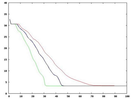
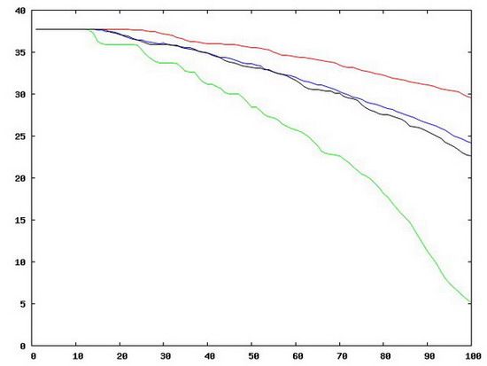
1. Let's assign p = (0; 5; -5; 1). This means a 5 pixel translation along the X axis and a (-5) pixel translation along the Y axis. The graph is shown below. The X axis contains the iteration numbers and the Y axis contains the mean error values for each iteration.

Let's assign  p = (0.01; 0; 0; 1). This means some in-plane rotation. The graph is placed below. The X axis contains the iteration numbers and the Y axis contains the mean error values for each iteration.

Let's assign  p = (0; 0; 0; 1.05). This means some scaling. The graph is placed below. The X axis contains the iteration numbers and the Y axis contains the mean error values for each iteration.

What can we see from the graphs above?

1. The algorithms work well in all three experiments, and search for the local minimum of the similarity function, .
2. In graph 2, we can see that the inverse compositional method oscillates. We can avoid the oscillations if we add the additional termination criteria.
3. In graphs 1 and 2, the algorithms converge quickly, and almost half of the iterations are not needed, because the mean error value is not decreased on them. So, we definitely need another termination criteria to avoid such unneeded iterations.

Now, let's compare which algorithm runs faster.

Experiment number	Algorithm name	Calculation time, sec.	Iteration count	Resulting mean error
1	Forwards additive	0.859	100	3.328212
	Inverse additive	0.594	100	3.337578
	Forwards comp.	1.078	100	3.367346
	Inverse comp.	0.469	100	3.341545
2	Forwards additive	0.875	100	3.397880
	Inverse additive	0.579	100	3.395847
	Forwards comp.	1.093	100	3.395613
	Inverse comp.	0.453	100	7.059829
3	Forwards additive	0.859	100	5.087051
	Inverse additive	0.594	100	24.136780
	Forwards comp.	1.11	100	29.541159
	Inverse comp.	0.469	100	22.628626

From the table above, we see that:

1. The fastest algorithms are the inverse additive and the inverse compositional ones. The slowest one is the forwards compositional algorithm.
2. All algorithms reach a maximum iteration count (100). Maybe, we should increase the MAX_ITER constant, which is the maximum available iterations number.
3. The resulting mean error is big in the third experiment for all the algorithms except the forwards additive. This means the template and image I are too different, so more iterations are needed for convergence (or they may not converge at all). If we increase the MAX_ITER constant, it is possible that the resulting mean error would be smaller.

Conclusion

In this article, we implemented the forwards compositional and the Hager-Belhumeur inverse additive image alignment algorithms. We slightly modified the code of the algorithms that we already implemented in Part I of this article. We compared the performance and the convergence speed of all the implemented algorithms in three simple experiments.

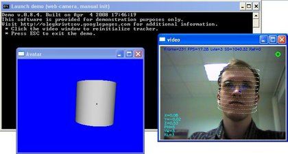
Is it possible to build real-time applications based on one of these algorithms? Many researchers say yes. For example, J. Xiao et al. created the system that was able to work at a speed of about 15 FPS. Their method is very similar to the forwards compositional algorithm.

We tried to use some techniques proposed by J. Xiao and his colleagues in our own head tracking system, and here you can find the demo. On my machine (Pentium IV 3GHz), it works at about 15 FPS. The usage of the inverse compositional method promises an even better speed.

License

This article, along with any associated source code and files, is licensed under The Code Project Open License (CPOL)