吴恩达深度学习笔记（一）——神经网络基础、 logistic 回归

观看了吴恩达老师的深度学习公开课，总结了部分个人觉得有益的知识点。

参考链接

一、数据结构
当编写神经网络程序时，就不要用这种秩为1的数据结构，如shape等于(n, )，或者是一维数组时。

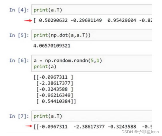
两对方括号和一对方括号，这就是1行5列的矩阵和一维数组的差别。

二.隐藏层的含义

三、L1W2作业

3.1 作业代码

参考链接1
参考链接2

import numpy as np
import matplotlib.pyplot as plt
import h5py
import scipy
from PIL import Image
from scipy import ndimage
from lr_utils import load_dataset

# load data
train_set_x_orig, train_set_y, test_set_x_orig, test_set_y, classes = load_dataset()

# 图片预览
index = 2
print(train_set_x_orig[index].shape)
plt.imshow(train_set_x_orig[index])
plt.show()

#打印出当前的训练标签值
#使用np.squeeze的目的是压缩维度，【未压缩】train_set_y[:,index]的值为[1] , 【压缩后】np.squeeze(train_set_y[:,index])的值为1
#print("【使用np.squeeze：" + str(np.squeeze(train_set_y[:,index])) + "，不使用np.squeeze： " + str(train_set_y[:,index]) + "】")
#只有压缩后的值才能进行解码操作
print("y=" + str(train_set_y[:,index]) + ", it's a '" + classes[np.squeeze(train_set_y[:,index])].decode("utf-8") + "' picture")

# 获取数据维度信息
print(train_set_x_orig.shape) # (209, 64, 64, 3)
print(train_set_y.shape) # (1, 209)
print(test_set_x_orig.shape) # (50, 64, 64, 3)
print(test_set_y.shape) # (1, 50)

m_train = train_set_y.shape[1]
m_test = test_set_y.shape[1]
num_px = test_set_x_orig.shape[1]

print("训练集的样本数："+str(m_train))
print("测试集的样本数："+str(m_test))
print("图片的宽和高："+str(num_px))

# 更改原数据的形状
# numpy使用reshape时，会先从axis=0填充数据，故用博主的方式可以保证每一行(转置后的每一列)的数据都来自同一图片
# train_set_x_flatten = train_set_x_orig.reshape(-1,train_set_x_orig.shape[0])
train_set_x_flatten = train_set_x_orig.reshape(train_set_x_orig.shape[0], -1).T
print(train_set_x_flatten.shape)
# test_set_x_flatten = test_set_x_orig.reshape(-1, test_set_x_orig.shape[0])
test_set_x_flatten = test_set_x_orig.reshape(test_set_x_orig.shape[0], -1).T
print(test_set_x_flatten.shape)

# 标准化数据集
train_set_x = train_set_x_flatten /255
test_set_x = test_set_x_flatten /255

# 定义激活函数
def sigmoid(z):
    s = 1/(1+np.exp(-z))
    return s

# 初始化模型参数
def initialize_params(dim):

    #W = np.random.normal(0,0.01,(train_set_x.shape[0],1))
    #b = np.zeros((1,m_train))
    W = np.zeros((dim, 1))
    b = 0
    # 使用断言确保数据正确
    assert(W.shape == (dim, 1))
    assert(isinstance(b, float) or isinstance(b, int))

    return W, b


# 传播函数
def propagate(W, b, X, y):

    m = X.shape[1]
    # 正向传播
    Z = np.dot(W.T, X) + b
    A = sigmoid(Z)
    J = np.sum(-y*np.log(A)-(1-y)*np.log(1-A))/m
    # 反向传播
    dZ = A - y
    dw = np.dot(X, dZ.T) / m
    db = np.sum(dZ) / m

    grads = {"dw": dw, "db": db}  #用字典来保存

    return J, grads

# 更新参数
def optimizer(W, b, X, y, num_iterations, lr, show_cost):

    cost_ls = []
    for i in range(num_iterations):
        cost, grads = propagate(W, b, X, y)
        dw = grads["dw"]
        db = grads["db"]
        W = W - lr*dw
        b = b - lr*db

        if i % 100 == 0:
            cost_ls.append(cost)

        if(show_cost) and (i % 100 == 0):
            print(i,"----->",cost)

    params = {"W":W, "b":b}
    grads = {"dw": dw, "db": db}

    return params, grads, cost_ls

# 预测函数
def predict(W, b, X):

    m = X.shape[1]
    A = sigmoid(np.dot(W.T, X) + b)
    y_pred = np.zeros((1, m))
    for i in range(A.shape[1]):
        y_pred[0, i] = 1 if A[0, i] >= 0.5 else 0

    return y_pred

# 整合成一个函数
def model(X_train, y_train, X_test, y_test, num_iterations=2000, lr=0.5, show_cost=False):  # 学习率设置过大，或导致内存溢出，出现nan

    W, b = initialize_params(X_train.shape[0])
    params, grads, cost_ls = optimizer(W, b, X_train, y_train, num_iterations, lr, show_cost)

    W = params["W"]
    b = params["b"]

    y_pred_train = predict(W, b, X_train)
    y_pred_test = predict(W, b, X_test)

    print("训练集准确性：", format(100-np.mean(np.abs(y_pred_train - y_train))*100),"%")  # 相同为0，不同为1
    print("测试集准确性：", format(100 - np.mean(np.abs(y_pred_test - y_test)) * 100), "%")

    d = {"cost_ls":cost_ls,"y_pred_train":y_pred_train, "y_pred_test":y_pred_test, "W":W, "b":b, "lr":lr}

    return d


d = model(train_set_x, train_set_y, test_set_x, test_set_y, num_iterations = 2000, lr = 0.005, show_cost = True)
print(d)

costs = d["cost_ls"]
plt.plot(costs)
plt.xlabel("iterations")
plt.ylabel("cost")
plt.show()

输出结果：

(64, 64, 3)
y=[1], it's a 'cat' picture
(209, 64, 64, 3)
(1, 209)
(50, 64, 64, 3)
(1, 50)
训练集的样本数：209
测试集的样本数：50
图片的宽和高：64
(12288, 209)
(12288, 50)
0 -----> 0.6931471805599453
100 -----> 0.5845083636993086
200 -----> 0.46694904094655465
300 -----> 0.3760068669480207
400 -----> 0.33146328932825125
500 -----> 0.3032730674743828
600 -----> 0.27987958658260487
700 -----> 0.26004213692587563
800 -----> 0.24294068467796612
900 -----> 0.2280042225672607
1000 -----> 0.21481951378449637
1100 -----> 0.2030781906064499
1200 -----> 0.1925442771670686
1300 -----> 0.18303333796883509
1400 -----> 0.17439859438448874
1500 -----> 0.1665213970540033
1600 -----> 0.15930451829756617
1700 -----> 0.15266732471296507
1800 -----> 0.14654223503982336
1900 -----> 0.14087207570310167
训练集准确性： 99.04306220095694 %
测试集准确性： 70.0 %
{'cost_ls': [0.6931471805599453, 0.5845083636993086, 0.46694904094655465, 0.3760068669480207, 0.33146328932825125, 0.3032730674743828, 0.27987958658260487, 0.26004213692587563, 0.24294068467796612, 0.2280042225672607, 0.21481951378449637, 0.2030781906064499, 0.1925442771670686, 0.18303333796883509, 0.17439859438448874, 0.1665213970540033, 0.15930451829756617, 0.15266732471296507, 0.14654223503982336, 0.14087207570310167], 'y_pred_train': array([[0., 0., 1., 0., 0., 0., 0., 1., 0., 0., 0., 1., 0., 1., 1., 0.,
        0., 0., 0., 1., 0., 0., 0., 0., 1., 1., 0., 1., 0., 1., 0., 0.,
        0., 0., 0., 0., 0., 0., 1., 0., 0., 0., 1., 0., 0., 0., 0., 1.,
        0., 0., 1., 0., 0., 0., 1., 0., 1., 1., 0., 1., 1., 1., 0., 0.,
        0., 0., 0., 0., 1., 0., 0., 1., 0., 0., 0., 1., 0., 0., 0., 0.,
        0., 0., 0., 1., 1., 0., 0., 0., 1., 0., 0., 0., 1., 1., 1., 0.,
        0., 1., 0., 0., 0., 0., 1., 0., 1., 0., 1., 1., 1., 1., 1., 1.,
        0., 0., 0., 0., 0., 1., 0., 0., 0., 1., 0., 0., 1., 0., 1., 0.,
        1., 1., 0., 0., 0., 1., 1., 1., 1., 1., 0., 0., 0., 0., 1., 0.,
        1., 1., 1., 0., 1., 1., 0., 0., 0., 1., 0., 0., 1., 0., 0., 0.,
        0., 0., 1., 0., 1., 0., 1., 0., 0., 1., 1., 1., 0., 0., 1., 1.,
        0., 1., 0., 1., 0., 0., 0., 0., 0., 1., 0., 0., 1., 0., 0., 0.,
        1., 0., 0., 0., 0., 1., 0., 0., 1., 0., 0., 0., 0., 0., 0., 0.,
        0.]]), 'y_pred_test': array([[1., 1., 1., 1., 1., 1., 0., 1., 1., 1., 0., 0., 1., 1., 0., 1.,
        0., 1., 0., 0., 1., 0., 0., 1., 1., 1., 1., 0., 0., 1., 0., 1.,
        1., 0., 1., 0., 0., 1., 0., 0., 1., 0., 1., 0., 1., 0., 0., 1.,
        1., 0.]]), 'W': array([[ 0.00961402],
       [-0.0264683 ],
       [-0.01226513],
       ...,
       [-0.01144453],
       [-0.02944783],
       [ 0.02378106]]), 'b': -0.01590624399969292}

3.2 将学习率lr设置的比较大的时候，会遇到RuntimeWarning: divide by zero encountered in log警告

参考链接

是因为sigmoid函数进行exp(-z)运算时，因为输入得z值太大（正值）或太小（负值），产生了内存溢出，最终得到的结果是nan。所以在cost函数中的log计算引发此警告。

比如将lr设置为0.5：

直接报错！

修改为0.005就正常了。

3.3 测试集的准确率始终为34%，而前面的代码经测试均没问题

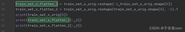
原因如下：

在修改原输入数据时，不能采用注释掉的那一种形式，而应该使用参考链接的，-1放在后面的形式。这是因为：numpy使用reshape时，会先从axis=0填充数据，故用博主的方式可以保证每一行(转置后的每一列)的数据都来自同一图片。而如果train_set_x_orig.shape[0]放在后面，则无法保证来自同一张图片。

下面观察这两种形式，第一列的输入特征（第一张图）有何不同：

第一张图片大概是：

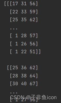
而两者的结果：

从结果来看，只有后者的数据才能保证来自同一图片。

修改后的预测结果：

3.4 尝试增加上面单元格中的迭代次数（修改为3000），可能会看到训练集准确性提高了，但是测试集准确性却降低了。 这称为过度拟合。

3.5 拎出一张图片查看预测结果

测试集第11张

# 图片对比查看
index_t = 10
plt.imshow(test_set_x[:,index_t].reshape((num_px, num_px, 3)))
plt.show()

print("y=" + str(test_set_y[:,index_t]) + ", You predicted that it is a '" + classes[int(d["y_pred_test"][:, index_t])].decode("utf-8") + "' picture")

然后就发现它预测错了。。。

3.6 超参数——学习率的选择

学习率决定我们更新参数的速度。 如果学习率太大，我们可能会“超出”最佳值。 同样，如果太小，将需要更多的迭代才能收敛到最佳值。

# 学习率的选择
learning_rates = [0.01, 0.001, 0.0001]
models = {}
for i in learning_rates:
    print ("learning rate is: " + str(i))
    models[str(i)] = model(train_set_x, train_set_y, test_set_x, test_set_y, num_iterations = 1500, lr = i, show_cost = False)
    print ('\n' + "-------------------------------------------------------" + '\n')

for i in learning_rates:
    plt.plot(np.squeeze(models[str(i)]["cost_ls"]), label= str(models[str(i)]["lr"]))

plt.ylabel('cost')
plt.xlabel('iterations')

legend = plt.legend(loc='upper center', shadow=True)
frame = legend.get_frame()   # 获得背景
frame.set_facecolor('0.90') # 设置背景透明度
plt.show()

结果：

learning rate is: 0.01
训练集准确性： 99.52153110047847 %
测试集准确性： 68.0 %

-------------------------------------------------------

learning rate is: 0.001
训练集准确性： 88.99521531100478 %
测试集准确性： 64.0 %

-------------------------------------------------------

learning rate is: 0.0001
训练集准确性： 68.42105263157895 %
测试集准确性： 36.0 %

-------------------------------------------------------


Process finished with exit code 0

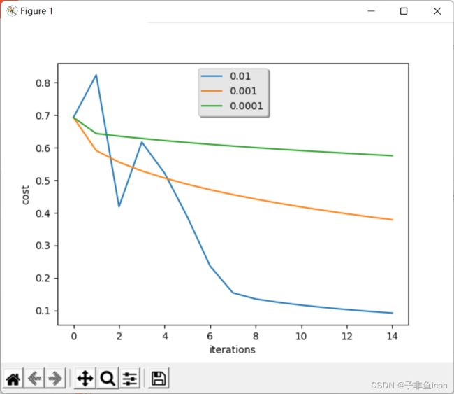
不同的学习率会带来不同的损失，因此会有不同的预测结果。

如果学习率太大（0.01），则成本可能会上下波动。 它甚至可能会发散（尽管在此示例中，使用0.01最终仍会以较高的损失值获得收益）。
较低的损失并不意味着模型效果很好。当训练精度比测试精度高很多时，就会发生过拟合情况。

在深度学习中，通常建议：
1.选择好能最小化损失函数的学习率。
2.如果模型过度拟合，请使用其他方法来减少过度拟合。

3.7 使用其他的猫猫图

网上下载的：

程序：

# 使用其他的猫猫图
fname = "D:\PyCharm files\deep learning\吴恩达\L1W2\cat.jpeg"
image = np.array(plt.imread(fname))
print(image.shape)

from skimage.transform import resize

my_image = resize(image,output_shape=(num_px,num_px))  # 修改尺寸为64*64
plt.imshow(my_image)
plt.show()

my_image = my_image.reshape((1, num_px*num_px*3)).T  # 转换成向量便于预测
print(my_image.shape)
#my_image = scipy.misc.imresize(image, size=(num_px,num_px)).reshape((1, num_px*num_px*3)).T
my_predicted_image = predict(d["W"], d["b"], my_image)
print("y = " + str(np.squeeze(my_predicted_image)) + ", your algorithm predicts a \"" + classes[int(np.squeeze(my_predicted_image)),].decode("utf-8") +  "\" picture.")

此处按照参考链接的可能会报错，是因为scipy的版本问题。参考链接

经过程序修改尺寸为64×64后

输出：

(220, 176, 3)
(12288, 1)
[[0.]]
y = 0.0, your algorithm predicts a "non-cat" picture.

嗯…识别失败，证明这个神经网络模型，的确有待提高。