机器学习算法入门梳理——逻辑回归的分类预测详解
基于逻辑回归的分类预测
机器学习算法详解,day1 打卡!
- 逻辑回归概述及函数
- 逻辑回归的python实现
- sklearn实现二分类逻辑回归
- 决策边界
- 适用多项式特征
- 多分类问题
- 总结
1. 逻辑回归概述及函数
1.1 概述
逻辑回归(logistic regression)是在数据科学领域最常用到的方法之一,虽然名字为“回归”,但逻辑回归其实是一个分类模型,主要是解决分类问题。
在逻辑回归中,我们会得到一个事件的概率值 p,当 p >= 0.5 时,事件发生;当 p < 0.5 时,事件不发生。
y = { 1 , p ^ ≥ 0.5 0 , p ^ ≤ 0.5 y=\left\{ \begin{array}{lr} 1, \ \ \hat{p}\geq0.5\\ 0, \ \ \hat{p}\leq0.5\\ \end{array} \right. y={1, p^≥0.50, p^≤0.5
1.2 函数表示
在线性回归中,估计值y为:
y ^ = θ T ⋅ x b \hat{y}=\theta^T \cdot x_b y^=θT⋅xb
这样得到的y值值域为 [-inf,inf] ,而概率的值域为[0,1]。因此我们想引入一个 σ \sigma σ , 使得函数值的值域在0到1之间,从而更方便地改变概率值。
p ^ = σ ( θ T ⋅ x b ) \hat{p}= \sigma\left(\theta^T \cdot x_b\right) p^=σ(θT⋅xb)
而这个 σ \sigma σ 我们一般用 Sigmoid 函数:
σ ( t ) = 1 1 + e − t \sigma\left(t\right)=\frac{1}{1+e^{-t}} σ(t)=1+e−t1
# Sigmoid函数

import numpy as np
import matplotlib.pyplot as plt

def sigmoid(t):
    return 1/(1+np.exp(-t))

x = np.arange(-10, 10, 0.1)
y = sigmoid(x)

plt.plot(x, y)
plt.show()
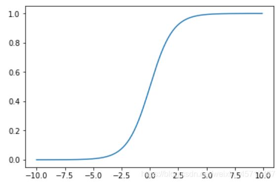
这个函数的值域在(0,1)之间;当 t > 0 时,p > 0.5 ; 当 t < 0 时,p < 0.5 。
当我们把 sigmoid 函数中的 t 替换为线性函数时:
p ^ = σ ( θ T ⋅ x b ) = 1 1 + e − θ T ⋅ x b \hat{p}= \sigma\left(\theta^T \cdot x_b\right)=\frac{1}{1+e^{-\theta^T \cdot x_b}} p^=σ(θT⋅xb)=1+e−θT⋅xb1
1.3 损失函数的推导和求解
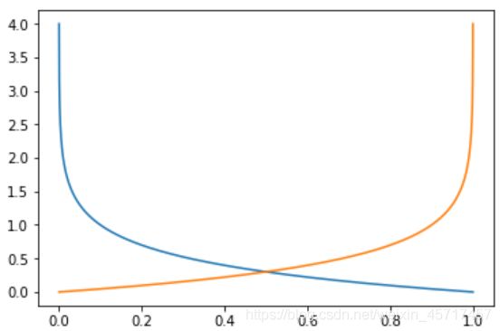
从上述公式中,我们可以看出对于一组数据 X ,要想预测出 y ,那么需要知道 θ \theta θ 的值。当损失函数最小时,对应的 θ \theta θ 也就是我们想找的了。当真实情况(y)为1时,预测的 p 越小,则 cost 越大;y 是 0 时,预测的 p 越大,则 cost 越大。什么样的函数满足呢?
c o s t = { − l o g ( p ^ ) , y = 1 − l o g ( 1 − p ^ ) , y = 0 cost=\left\{ \begin{array}{lr} -log\left(\hat{p}\right), \ \ \ \ \ \ \ \ \ \ y=1\\ -log\left(1-\hat{p}\right), \ \ \ y=0\\ \end{array} \right. cost={−log(p^), y=1−log(1−p^), y=0
这个cost函数的图像为( p 只能在 [0, 1] 之间取值):
import math
x = np.arange(0.0001, 1, 0.0001)
y1 = [-(math.log10(i)) for i in x]
y2 = [-(math.log10(1-i)) for i in x]


fig,ax = plt.subplots()

plt.plot(x , y1)
plt.plot(x , y2)
plt.show()
由于这样分类讨论并不方便,因此可以将这两部分合为一个函数:
c o s t = − y l o g ( p ^ ) − ( 1 − y ) ( 1 − p ^ ) cost=-ylog\left(\hat{p}\right)-\left(1-y\right)\left(1-\hat{p}\right) cost=−ylog(p^)−(1−y)(1−p^)
对于多个样本而言,损失函数为:
J ( θ ) = − 1 m ∑ i = 1 m y ( i ) l o g ( p ^ ( i ) ) + ( 1 − y ( i ) ) ( 1 − p ^ ( i ) ) J\left(\theta\right)=-\frac{1}{m}\sum_{i=1}^{m} y^{\left(i\right)}log\left(\hat{p}^{\left(i\right)}\right)+\left(1-y^{\left(i\right)}\right)\left(1-\hat{p}^{\left(i\right)}\right) J(θ)=−m1i=1∑my(i)log(p^(i))+(1−y(i))(1−p^(i))
即:
J ( θ ) = − 1 m ∑ i = 1 n y ( i ) l o g ( σ ( X b ( i ) θ ) ) + ( 1 − y ( i ) ) ( 1 − σ ( X b ( i ) θ ) ) J\left(\theta\right)=-\frac{1}{m}\sum_{i=1}^{n} y^{\left(i\right)}log\left(\sigma\left(X_b^{\left(i\right)}\theta\right)\right)+\left(1-y^{\left(i\right)}\right)\left(1-\sigma\left(X_b^{\left(i\right)}\theta\right)\right) J(θ)=−m1i=1∑ny(i)log(σ(Xb(i)θ))+(1−y(i))(1−σ(Xb(i)θ))
这个损失函数没有公式解 θ \theta θ 使得 J ( θ ) J\left(\theta\right) J(θ) 最小,但是可以通过梯度下降法求解。由于这是一个凸函数,所以不用考虑局部最优解,只有一个全局最优解。
由于函数比较复杂,先对sigmoid函数进行求导得到:
σ ( t ) = ( 1 + e − t ) − 1 \sigma\left(t\right)=\left(1+e^{-t}\right)^{-1} σ(t)=(1+e−t)−1
σ ′ ( t ) = ( 1 + e − t ) − 2 ⋅ e − t \sigma^{'}\left(t\right)=\left(1+e^{-t}\right)^{-2} \cdot e^{-t} σ′(t)=(1+e−t)−2⋅e−t
(在这里写公式很麻烦,所以此处只能粘贴了)
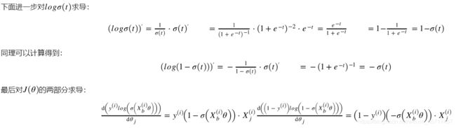
两者相加,整理可得:
( y ( i ) − σ ( X b ( i ) θ ) ) ⋅ X j ( i ) \left(y^{\left(i\right)} - \sigma\left(X_b^{\left(i\right)}\theta\right)\right) \cdot X_j^{\left(i\right)} (y(i)−σ(Xb(i)θ))⋅Xj(i)
所以 J ( θ ) J\left(\theta\right) J(θ) 的导数为:
J ( θ ) θ j a m p ; = 1 m ∑ i = 1 m ( σ ( X b ( i ) θ ) − y ( i ) ) X j ( i ) a m p ; = 1 m ∑ i = 1 m ( y ^ ( i ) − y ( i ) ) X j ( i ) \begin{aligned} \frac{J\left(\theta\right)}{\theta_j}&=\frac{1}{m}\sum_{i=1}^{m}\left(\sigma\left(X_b^{\left(i\right)}\theta\right)-y^{\left(i\right)}\right)X_j^{\left(i\right)}\\ &=\frac{1}{m}\sum_{i=1}^{m}\left(\hat{y}^{\left(i\right)} - y^{\left(i\right)}\right)X_j^{\left(i\right)} \end{aligned} θjJ(θ)amp;=m1i=1∑m(σ(Xb(i)θ)−y(i))Xj(i)amp;=m1i=1∑m(y^(i)−y(i))Xj(i)
可以看到与线性回归很像,只是 y ^ \hat{y} y^ 在线性回归的基础上套了 sigmoid 函数。
∇ J ( θ ) = 1 m ⋅ X b T ⋅ ( σ ( X b θ ) − y ) \nabla J\left(\theta\right)=\frac{1}{m} \cdot X_b^T \cdot \left(\sigma\left(X_b\theta\right)-y\right) ∇J(θ)=m1⋅XbT⋅(σ(Xbθ)−y)
2. 逻辑回归的python实现
下面是对应的code及调用:
import warnings
warnings.filterwarnings('ignore')

import numpy as np
from sklearn.metrics import accuracy_score

class LogisticRegression:

    def __init__(self):
        self.coef = None
        self.intercept = None
        self.theta = None

    # 定义sigmoid函数
    def sigmoid(self, t):
        return 1/(1 + np.exp(-t))

    # 梯度下降法
    def fit(self, X_train, Y_train, eta = 0.01, n_iters = 1e4):

        X_b = np.hstack([np.ones((len(X_train), 1)), X_train]) # 初始向量X_b比X_train是多一列1
        initial_theta = np.zeros(X_b.shape[1]) # 初始theta

        def J(theta, X_b, y):
            y_hat = self.sigmoid(X_b.dot(theta))
            return -np.sum(y * np.log(y_hat) + (1-y) * np.log(1-y_hat))/len(X_b)

        # 求导
        def dJ(theta, X_b, y):
            return X_b.T.dot(self.sigmoid(X_b.dot(theta)) - y)/len(X_b)

        # 梯度下降
        def gradent_descent(X_b, y, initial_theta, eta, n_iters=1e4, epsilon=1e-8):
            theta = initial_theta
            cur_iter = 0

            while cur_iter < n_iters:
                gradient = dJ(theta, X_b, y)
                last_theta = theta
                theta = theta - eta * gradient

                if abs(J(theta, X_b, y) - J(last_theta, X_b, y)) < epsilon:
                    break

                cur_iter += 1

            return theta

        self.theta = gradent_descent(X_b, Y_train, initial_theta, eta, n_iters)
        self.intercept = self.theta[0]
        self.coef = self.theta[1:]

        return self

    # 预测概率
    def predict_prob(self, X_predict):
        X_b = np.hstack([np.ones((len(X_predict), 1)), X_predict])
        return self.sigmoid(X_b.dot(self.theta))

    # 返回预测值
    def predict(self, X_predict):
        prob = self.predict_prob(X_predict)
        return np.array(prob >= 0.5, dtype='int') # True -> 1 ; False -> 0

    # 得到accuracy score
    def score(self, X_test, y_test):
        y_predict = self.predict(X_test)
        return accuracy_score(y_test, y_predict)
# 使用iris数据测试
from sklearn.model_selection import train_test_split
from sklearn import datasets
iris = datasets.load_iris()

# 由于LR适用于二分类问题,而iris有三组预测值,所以先去掉一组
X = iris.data
y = iris.target

X = X[y<2,:2]
y = y[y<2]

# 使用上面写的逻辑回归预测
X_train, X_test, y_train, y_test = train_test_split(X, y)
LR = LogisticRegression()

# 训练
LR.fit(X_train, y_train)

# 参数
# print(LR.coef)
# print(LR.theta)
# print(LR.intercept)

# 概率
print(LR.predict_prob(X_test))

# 预测结果
print(LR.predict(X_test))

# 分数
LR.score(X_test, y_test)
[0.97686488 0.97164471 0.97686488 0.98597419 0.97438396 0.92545021
 0.16039916 0.00594648 0.99814416 0.16039916 0.98603084 0.10331793
 0.08551181 0.03959817 0.13470587 0.59376965 0.00290751 0.99657567
 0.98580286 0.98091347 0.93863763 0.87041905 0.96542582 0.0531791
 0.93816306]
[1 1 1 1 1 1 0 0 1 0 1 0 0 0 0 1 0 1 1 1 1 1 1 0 1]
out: 1.0
3. sklearn实现二分类逻辑回归
from sklearn.model_selection import train_test_split
from sklearn.linear_model import LogisticRegression
from sklearn.metrics import accuracy_score, confusion_matrix
import seaborn as sns
from sklearn import datasets
iris = datasets.load_iris()
X = iris.data
y = iris.target
X = X[y<2]
y = y[y<2]
X_train, X_test, y_train, y_test = train_test_split(X, y)
# 训练
clf = LogisticRegression()
clf.fit(X_train, y_train)
test_predict = clf.predict(X_test)
# 预测的accuracy达到了1
accuracy_score(y_test, test_predict)
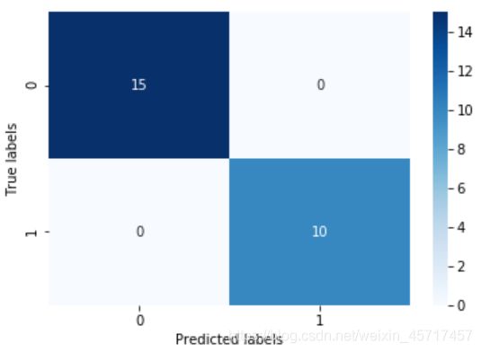
confusion_matrix_result = confusion_matrix(test_predict,y_test)
sns.heatmap(confusion_matrix_result, annot=True, cmap='Blues')
plt.xlabel('Predicted labels')
plt.ylabel('True labels')
plt.show()
4. 决策边界
对于分类问题,决策边界一个很关键的问题。在 sigmoid 函数中,当 t >= 0.5 时,预测概率 p >= 0.5;而 t < 0 时,预测概率 p < 0.5 。而这个 t 也就是 θ T ⋅ x b \theta^T \cdot x_b θT⋅xb 。
y = { 1 , p ^ ≥ 0.5 θ T ⋅ x b ≥ 0.5 0 , p ^ < 0.5 θ T ⋅ x b < 0.5 y=\left\{ \begin{array}{lr} 1, \ \hat{p}\geq0.5 \ \ \ \ \theta^T \cdot x_b \geq 0.5\\ 0, \ \hat{p}<0.5 \ \ \ \ \theta^T \cdot x_b < 0.5\\ \end{array} \right. y={1, p^≥0.5 θT⋅xb≥0.50, p^<0.5 θT⋅xb<0.5
θ T ⋅ x b \theta^T \cdot x_b θT⋅xb = 0,也就是决策边界。假如 X 有两个特征,也就是 θ 0 \theta_0 θ0 + θ x 1 \theta x_1 θx1 + θ 2 x 2 \theta_2x_2 θ2x2 = 0,可解得:
x 2 = − θ 0 − θ 1 x 1 θ 2 x_2=\frac{-\theta_0 - \theta_1x_1}{\theta_2} x2=θ2−θ0−θ1x1
# 计算x2

def cal_x2(x1):
    return - (LR.coef[0] * x1 - LR.intercept)/LR.coef[1]

X = iris.data
y = iris.target

# 只用两个特征可视化:
X = X[y<2,:2]
y = y[y<2]

x1_plot = np.linspace(4,8,1000)
x2_plot = cal_x2(x1_plot)

plt.scatter(X[y==0,0], X[y==0,1], color = 'red')
plt.scatter(X[y==1,0], X[y==1,1], color = 'green')
plt.plot(x1_plot, x2_plot, color = 'blue')
plt.show()
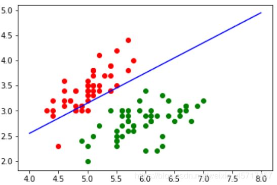
从上图可以看到,这两个 target 被分成了两部分。但是之前我们的预测 score 是 1 ,应该全部都对,但是目前红点有判断错误的。这是因为这是用的全部数据,而打分的时候用的是 test 的数据。对于正好在边界的数据,我们分成哪一类都可以。
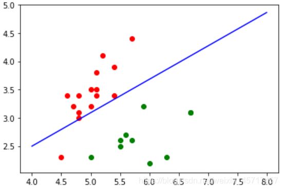
plt.scatter(X_test[y_test==0,0], X_test[y_test==0,1], color = 'red')
plt.scatter(X_test[y_test==1,0], X_test[y_test==1,1], color = 'green')
plt.plot(x1_plot, x2_plot, color = 'blue')
plt.show()
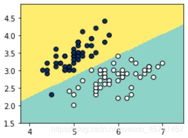
# 直接写一个画边界的函数

def plot_boundary(model, X, y):
    x_min, x_max = X[:, 0].min() - .5, X[:, 0].max() + .5
    y_min, y_max = X[:, 1].min() - .5, X[:, 1].max() + .5

    h = .02  # step size in the mesh
    xx, yy = np.meshgrid(np.arange(x_min, x_max, h), np.arange(y_min, y_max, h))
    Z = model.predict(np.c_[xx.ravel(), yy.ravel()])

    # Put the result into a color plot
    Z = Z.reshape(xx.shape)
    plt.figure(1, figsize=(4, 3))
    plt.pcolormesh(xx, yy, Z, cmap=plt.cm.Set3_r)

    # Plot also the training points
    plt.scatter(X[:, 0], X[:, 1], c=y, edgecolors='k', cmap=plt.cm.Blues_r)
    plt.show()
plot_boundary(LR, X, y)
5. 使用多项式特征
np.random.seed(1)
X = np.random.normal(0,1,size = (200,2))
y = np.array(X[:,0] ** 2 + X[:,1]**2 < 1.5, dtype='int')
plt.scatter(X[y==0,0], X[y==0,1], color = 'red')
plt.scatter(X[y==1,0], X[y==1,1], color = 'green')
plt.show()
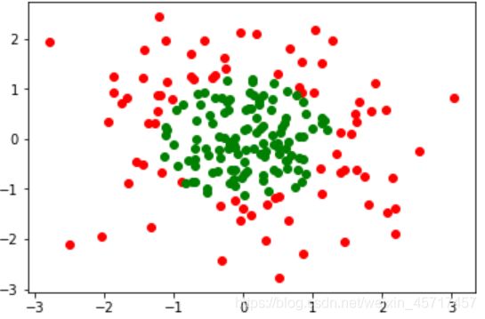
LR = LogisticRegression()

LR.fit(X,y)
LR.score(X,y)
out: 0.6
plot_boundary(LR, X, y)
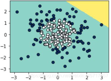
这样分类的效果是很一般的。下面用 sklearn 为逻辑回归增加多项式特征:
from sklearn.pipeline import Pipeline
from sklearn.preprocessing import PolynomialFeatures, StandardScaler

# 必须符合scikit_learn的标准才可以用

def PolynomialLR(degree):
    return Pipeline([
    ('poly', PolynomialFeatures(degree=degree)),
    ('std_scaler', StandardScaler()),
    ('LR', LogisticRegression())
    ])

# 调用
poly_LR = PolynomialLR(degree = 2)
poly_LR.fit(X,y)
poly_LR.score(X,y)
out: 0.955
plot_boundary(poly_LR, X, y)
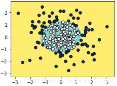
由此可见,这样的效果比之前好了许多。
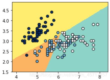
6. 多分类问题
常用的有两种方式:
1). OvR (One vs Rest)
每次将某个与剩下的所有的分类,
n 个类别进行 n 次分类,选择分类得分最高的。
2). OvO (One vs One)
两两组合,比如四个类别有六个组,选择赢数最高的分类。
from sklearn.linear_model import LogisticRegression

# 只使用前两种feature,方便可视化

X = iris.data[:,:2]
y = iris.target

X_train, X_test, y_train, y_test = train_test_split(X, y)

scikit_LR = LogisticRegression()

# 默认multi_class='ovr',即OVR
scikit_LR.fit(X_train, y_train)
scikit_LR.score(X_test, y_test)
out: 0.7631578947368421
plot_boundary(scikit_LR, X,y)
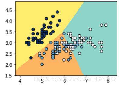
# 修改为OVO

# 修改 multi_class='multinomial';需要注意的是,solver也需要改变,scikit_learn不仅仅使用梯度下降法,默认是使用liblinear的,但是对于OVO是实效的
scikit_LR2 = LogisticRegression(multi_class='multinomial', solver='newton-cg')

scikit_LR2.fit(X_train, y_train)
scikit_LR2.score(X_test, y_test)
out: 0.8947368421052632
plot_boundary(scikit_LR2, X,y)
7. 总结
逻辑回归(Logistic regression,简称LR)虽然其中带有"回归"两个字,但逻辑回归其实是一个分类模型,并且广泛应用于各个领域之中。虽然现在深度学习相对于这些传统方法更为火热,但实则这些传统方法由于其独特的优势依然广泛应用于各个领域中。
而对于逻辑回归而言,最为突出的两点就是其模型简单和模型的可解释性强。
逻辑回归模型的优劣势:
优点:实现简单,易于理解和实现;计算代价不高,速度很快,存储资源低;
缺点:容易欠拟合,分类精度可能不高。
逻辑回归模型广泛用于各个领域,包括机器学习,大多数医学领域和社会科学。例如,最初由Boyd 等人开发的创伤和损伤严重度评分(TRISS)被广泛用于预测受伤患者的死亡率,使用逻辑回归 基于观察到的患者特征(年龄,性别,体重指数,各种血液检查的结果等)分析预测发生特定疾病(例如糖尿病,冠心病)的风险。逻辑回归模型也用于预测在给定的过程中,系统或产品的故障的可能性。还用于市场营销应用程序,例如预测客户购买产品或中止订购的倾向等。在经济学中它可以用来预测一个人选择进入劳动力市场的可能性,而商业应用则可以用来预测房主拖欠抵押贷款的可能性。条件随机字段是逻辑回归到顺序数据的扩展,用于自然语言处理。
逻辑回归模型现在同样是很多分类算法的基础组件,比如 分类任务中基于GBDT算法+LR逻辑回归实现的信用卡交易反欺诈,CTR(点击通过率)预估等,其好处在于输出值自然地落在 0 到 1 之间,并且有概率意义。模型清晰,有对应的概率学理论基础。它拟合出来的参数就代表了每一个特征(feature)对结果的影响。也是一个理解数据的好工具。但同时由于其本质上是一个线性的分类器,所以不能应对较为复杂的数据情况。很多时候我们也会拿逻辑回归模型去做一些任务尝试的基线(基础水平)。
参考资料:
1、阿里云notebook: https://developer.aliyun.com/ai/scenario/9ad3416619b1423180f656d1c9ae44f7
2、github地址:https://github.com/Liying1996/machine_learining/blob/master/Logistic_regression.ipynb