分类模型计算混淆矩阵

1. 什么是混淆矩阵

混淆矩阵是评判模型结果的一种指标，属于模型评估的一部分，常用于评判分类器的优劣。即，混淆矩阵是评判模型结果的指标，属于模型评估的一部分。

此外，混淆矩阵多用于判断分类器（Classifier）的优劣，适用于分类型的数据模型，如

• 分类树（Classification Tree）
• 逻辑回归（Logistic Regression）
• 线性判别分析（Linear Discriminant Analysis）等方法。

一句话解释版本：混淆矩阵就是分别统计分类模型归错类，归对类的观测值个数，然后把结果放在一个表里展示出来。这个表就是混淆矩阵。

---

在分类型模型评判的指标中，常见的方法有如下三种：

• 混淆矩阵（也称误差矩阵，Confusion Matrix）
• ROC曲线
• AUC面积

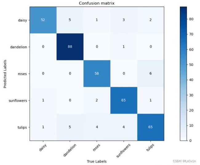
对于这个混淆矩阵，横坐标是真实标签（Ground Truth），纵坐标是模型预测的类别。对角线是我们最关注的信息，对角线代表预测正确的样本的个数。

	Precision (精确率)	Recall (召回率)	Specificity (特异度)
类别1	0.825	0.963	0.965
类别2	0.989	0.898	0.996
类别3	0.906	0.892	0.980
…	…	…	…

注意：准确率(accuracy)和精确率(precision)不是一回事，准确率一般用于分类网络，而精确率用于目标检测。

2. 混淆矩阵前置知识

2.1 混淆矩阵的定义

混淆矩阵（Confusion Matrix），它的本质远没有它的名字听上去那么拉风。矩阵，可以理解为就是一张表格，混淆矩阵其实就是一张表格而已。

以分类模型中最简单的二分类为例，对于这种问题，我们的模型最终需要判断样本的结果是0还是1，或者说是positive还是negative。我们通过样本的采集，能够直接知道真实情况下，哪些数据结果是positive，哪些结果是negative。同时，我们通过用样本数据跑出分类模型的结果，也可以知道模型认为这些数据哪些是positive，哪些是negative。

对于一个二分类网络，模型本质上只有1个类别，即模型的预测结果只有是这个类别（正样本）和不是这个类别（负样本）这两种结果。

因此，我们就能得到这样四个基础指标，我称他们是一级指标（最底层的）：

• 真实值是positive，模型认为是positive的数量（True Positive=TP） -> 真阳性
• 真实值是positive，模型认为是negative的数量（False Negative=FN）：这就是统计学上的第二类错误（Type II Error） -> 假阴性
• 真实值是negative，模型认为是positive的数量（False Positive=FP）：这就是统计学上的第一类错误（Type I Error） -> 假阳性
• 真实值是negative，模型认为是negative的数量（True Negative=TN） -> 真阴性

对于二分类网络，1 代表的就是Positive, 0 代表的就是Negative。

---

注意： Positive和Negative是针对网络的预测结果得到的，和真实值无关，真实值和True/False有关。

• 模型预测的是1（Positive），与GT相符 -> TP -> 真阳性
• 模型预测的是1（Positive），与GT不符 -> FP -> 假阳性
• 模型预测的是0（Negative），与GT相符 -> TN -> 真阴性
• 模型预测的是0（Negative），与GT不符 -> FN -> 假阴性

将这四个指标一起呈现在表格中，就能得到如下这样一个矩阵，我们称它为混淆矩阵（Confusion Matrix）：

对于左上角的混淆矩阵来说，同样的，每一行代表真实值的标签，每一列代表预测值的标签。

• Positive: 正样本（真实值）
• Negative：负样本（预测值）

2.2 混淆矩阵的指标

预测性分类模型，肯定是希望越准越好。那么，对应到混淆矩阵中，那肯定是希望TP与TN的数量大（预测值和GT一致的情况），而FP与FN的数量小（预测值与GT不符的情况）。所以当我们得到了模型的混淆矩阵后，就需要去看有多少观测值在第二、四象限对应的位置，这里的数值越多越好；反之，在第一、三象限对应位置出现的观测值肯定是越少越好。

• TP和TN越高越好
• FP和FN越少越好

2.3 二级指标——准确率、精确率、灵敏度/召回率、特异度

但是，混淆矩阵里面统计的是个数，有时候面对大量的数据，光凭算个数，很难衡量模型的优劣。混淆矩阵是直接把所有的数据都摆了上来，实际上并没有什么解读，所以需要一些指标来衡量混淆矩阵的好坏。

因此混淆矩阵在基本的统计结果上又延伸了如下4个指标，我们称它们为二级指标（通过最底层指标加减乘除得到的）：

• 准确率（Accuracy）—— 针对整个模型
• 精确率（Precision）
• 灵敏度（Sensitivity）：就是召回率（Recall）
• 特异度（Specificity）

二级指标	公式	描述	通俗解释
Accuracy (准确率)	$\mathrm{A}\mathrm{c}\mathrm{c}\mathrm{u}\mathrm{r}\mathrm{a}\mathrm{c}\mathrm{y}=\frac{\mathrm{T}\mathrm{P}+\mathrm{T}\mathrm{N}}{\mathrm{T}\mathrm{P}+\mathrm{F}\mathrm{P}+\mathrm{T}\mathrm{N}+\mathrm{F}\mathrm{N}}$	模型分类正确样本个数（正样本+负样本）占总样本个数的比例	所有正负样本中模型预测对的比例
Precision (精确率)	$\mathrm{P}\mathrm{r}\mathrm{e}\mathrm{c}\mathrm{i}\mathrm{s}\mathrm{i}\mathrm{o}\mathrm{n}=\frac{\mathrm{T}\mathrm{P}}{\mathrm{T}\mathrm{P}+\mathrm{F}\mathrm{P}}$	模型认为是正样本中，预测对的比例	模型认为是正样本中（不一定真的是正样本），预测对的比例
Recall (召回率/查全率)	$\mathrm{R}\mathrm{e}\mathrm{c}\mathrm{a}\mathrm{l}\mathrm{l}=\frac{\mathrm{T}\mathrm{P}}{\mathrm{T}\mathrm{P}+\mathrm{F}\mathrm{N}}$	所有真实的正样本中，模型预测对的比例	真实的正样本中预测了对了多少（模型本应该预测出来的正样本中预测了对了多少）
Specificity (特异度)	$\mathrm{S}\mathrm{p}\mathrm{e}\mathrm{c}\mathrm{i}\mathrm{f}\mathrm{i}\mathrm{c}\mathrm{i}\mathrm{t}\mathrm{y}=\frac{\mathrm{T}\mathrm{N}}{\mathrm{T}\mathrm{N}+\mathrm{F}\mathrm{P}}$	所有真实的负样本中，模型预测对的比例	真实的负样本中预测了对了多少（模型本应该预测出来的负样本中预测了对了多少）

通过上面的四个二级指标，可以将混淆矩阵中数量的结果转化为 $[0,1]$ 之间的比率，便于进行标准化的衡量。

在实际使用中，使用较多的是前三个指标（Accuracy, Precision, Recall）。

简单记忆：

• Accuracy: 模型预测的所有正负样本中，预测对了多少 —— 模型判断正确的数据(TP+TN)占总数据的比例
• Precision: 模型预测的所有正样本中，预测对了多少 —— Precision高表示模型检测出的正样本中大部分确实是正样本,只有少量不是正样本被当成正样本
• Recall: 模型本应该预测出来的正样本中预测了对了多少 —— 召回率也叫查全率,以目标检测为例,我们往往把图片中的物体作为正例，此时召回率高代表着模型可以找出图片中更多的物体!
• Specificity: 模型本应该预测出来的负样本中预测了对了多少 —— 特异度高代表着模型可以找出图片中更多的背景（负样本）!

2.4 三级指标

在这四个指标的基础上在进行拓展，会产令另外一个三级指标。这个指标叫做F1 Score。它的计算公式是：
$$\mathrm{F}1\mathrm{S}\mathrm{c}\mathrm{o}\mathrm{r}\mathrm{e}=\frac{2\mathrm{P}\mathrm{R}}{\mathrm{P}+\mathrm{R}}\in [0,1]$$

其中，P代表Precision，R代表Recall。

F1-Score指标综合了Precision与Recall的产出的结果。F1-Score的取值范围为[0, 1]：

• 1代表模型的输出最好
• 0代表模型的输出结果最差

3. 例子

3.1 准确率（Accuracy）

准确率简单来讲，就是对角线占所有的比例，即：
$$\begin{array}{rl}\text{Accuracy}& =\frac{\mathrm{T}\mathrm{P}+\mathrm{T}\mathrm{N}}{\mathrm{T}\mathrm{P}+\mathrm{F}\mathrm{P}+\mathrm{T}\mathrm{N}+\mathrm{F}\mathrm{N}}\\ & =\frac{10+15+20}{10+15+20+3+5+1+6+2+4}\\ & =\frac{10+15+20}{66}\\ & \approx 0.68\end{array}$$

所有正负样本中，预测对了多少

3.2 精确率（Precision）

对于精确率来说，我们以“猫”为例，3分类可以变为2分类——“猫”和“不为猫”。

$$\begin{array}{rl}\text{Precision}& =\frac{\mathrm{T}\mathrm{P}}{\mathrm{T}\mathrm{P}+\mathrm{F}\mathrm{P}}\\ & =\frac{10}{10+3}\\ & \approx 0.77\end{array}$$

模型预测的所有正样本中，预测对了多少

3.3 召回率（Recall）

$$\begin{array}{rl}\text{Recall}& =\frac{\mathrm{T}\mathrm{P}}{\mathrm{T}\mathrm{P}+\mathrm{F}\mathrm{N}}\\ & =\frac{10}{10+8}\\ & \approx 0.56\end{array}$$

模型本应该预测出来的正样本中预测了对了多少

3.4 特异度（Specificity）

$$\begin{array}{rl}\text{Specificity}& =\frac{\mathrm{T}\mathrm{P}}{\mathrm{T}\mathrm{P}+\mathrm{F}\mathrm{N}}\\ & =\frac{45}{45+3}\\ & \approx 0.94\end{array}$$

模型本应该预测出来的负样本中预测了对了多少

3.5 总结

对于二级指标来说：

• accuracy是可以根据所有类别来进行计算的（就是所有类别中，模型预测对的比例）
• 剩下的3个二级指标precision, recall, specificity就需要针对每一个类别进行计算（按照上面的例子那样做）。

4. 代码

代码来源于霹雳吧啦WZ老师。

import os
import json

import torch
from torchvision import transforms, datasets
import numpy as np
from tqdm import tqdm
import matplotlib.pyplot as plt
from prettytable import PrettyTable

from model import MobileNetV2


class ConfusionMatrix(object):
    """
    注意，如果显示的图像不全，是matplotlib版本问题
    本例程使用matplotlib-3.2.1(windows and ubuntu)绘制正常
    需要额外安装prettytable库  将输出打印为列表
    """
    def __init__(self, num_classes: int, labels: list):
        self.matrix = np.zeros((num_classes, num_classes))
        self.num_classes = num_classes
        self.labels = labels

    def update(self, preds, labels):
        for p, t in zip(preds, labels):  # p: predict, t: GT
            self.matrix[p, t] += 1

    def summary(self):
        # calculate accuracy
        sum_TP = 0
        for i in range(self.num_classes):
            sum_TP += self.matrix[i, i]
        acc = sum_TP / np.sum(self.matrix)
        print("the model accuracy is ", acc)

        # precision, recall, specificity
        table = PrettyTable()  # init a table for print
        table.field_names = ["", "Precision", "Recall", "Specificity"]
        for i in range(self.num_classes):  # for each class
            TP = self.matrix[i, i]
            FP = np.sum(self.matrix[i, :]) - TP
            FN = np.sum(self.matrix[:, i]) - TP
            TN = np.sum(self.matrix) - TP - FP - FN
            Precision = round(TP / (TP + FP), 3) if TP + FP != 0 else 0.
            Recall = round(TP / (TP + FN), 3) if TP + FN != 0 else 0.
            Specificity = round(TN / (TN + FP), 3) if TN + FP != 0 else 0.
            table.add_row([self.labels[i], Precision, Recall, Specificity])
        print(table)

    def plot(self):  # plot confusion matrix
        matrix = self.matrix
        print(matrix)
        plt.imshow(matrix, cmap=plt.cm.Blues)  # color from white to blue

        plt.xticks(range(self.num_classes), self.labels, rotation=45)
        plt.yticks(range(self.num_classes), self.labels)

        # show colorbar
        plt.colorbar()

        plt.xlabel('True Labels')
        plt.ylabel('Predicted Labels')
        plt.title('Confusion matrix')

        # 在图中标注数量/概率信息
        thresh = matrix.max() / 2
        # Note:
        #       x: left -> right; y: top -> bottom
        for x in range(self.num_classes):
            for y in range(self.num_classes):
                # 注意这里的matrix[y, x]不是matrix[x, y]
                info = int(matrix[y, x])
                plt.text(x, y, info,
                         verticalalignment='center',
                         horizontalalignment='center',
                         color="white" if info > thresh else "black")
        plt.tight_layout()
        plt.show()


if __name__ == '__main__':
    device = torch.device("cuda:0" if torch.cuda.is_available() else "cpu")
    print(device)

    data_transform = transforms.Compose([transforms.Resize(256),
                                         transforms.CenterCrop(224),
                                         transforms.ToTensor(),
                                         transforms.Normalize([0.485, 0.456, 0.406], [0.229, 0.224, 0.225])])

    data_root = os.path.abspath(os.path.join(os.getcwd(), "../.."))  # get data root path
    image_path = os.path.join(data_root, "data_set", "flower_data")  # flower data set path
    assert os.path.exists(image_path), "data path {} does not exist.".format(image_path)

    validate_dataset = datasets.ImageFolder(root=os.path.join(image_path, "val"),
                                            transform=data_transform)

    batch_size = 16
    validate_loader = torch.utils.data.DataLoader(validate_dataset,
                                                  batch_size=batch_size, shuffle=False,
                                                  num_workers=2)
    net = MobileNetV2(num_classes=5)
    # load pretrain weights
    model_weight_path = "./MobileNetV2.pth"
    assert os.path.exists(model_weight_path), "cannot find {} file".format(model_weight_path)
    net.load_state_dict(torch.load(model_weight_path, map_location=device))
    net.to(device)

    # read class_indict
    json_label_path = './class_indices.json'
    assert os.path.exists(json_label_path), "cannot find {} file".format(json_label_path)
    json_file = open(json_label_path, 'r')
    class_indict = json.load(json_file)

    labels = [label for _, label in class_indict.items()]
    confusion = ConfusionMatrix(num_classes=5, labels=labels)
    net.eval()
    with torch.no_grad():
        for val_data in tqdm(validate_loader):
            val_images, val_labels = val_data
            outputs = net(val_images.to(device))
            outputs = torch.softmax(outputs, dim=1)
            outputs = torch.argmax(outputs, dim=1)
            confusion.update(outputs.to("cpu").numpy(), val_labels.to("cpu").numpy())
    confusion.plot()
    confusion.summary()

参考

参考：

1. 使用pytorch和tensorflow计算分类模型的混淆矩阵_哔哩哔哩_bilibili
2. https://blog.csdn.net/Orange_Spotty_Cat/article/details/80520839