Poisson Disk Sampling
http://devmag.org.za/2009/05/03/poisson-disk-sampling/
This article originally appeared in Dev.Mag Issue 21, released in March 2008.
One way to populate large worlds with objects is to simply place objects on a grid, or randomly. While fast and easy to implement, both these methods result in unsatisfying worlds: either too regular or too messy. In this article we look at an alternative algorithm that returns a random set of points with nice properties:
- the points are tightly packed together; but
- no closer to each other than a specified minimum distance.
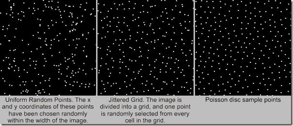
Figure 1 shows an example of such a set, which is called Poisson-disk sample set. For comparison, two other sample sets are also shown: a uniform random sample, and a jittered grid sample.
Poisson disk sampling has many applications in games:
- random object placement;
- sampling for graphics applications;
- procedural texture algorithms; and
- mesh algorithms.
In this article we will look mostly at object placement and briefly at texture generation.
Figure 1
Implementation
There are several algorithms for producing a Poisson disk sample set. The one presented here is easy to implement, and runs reasonably fast. It is also easy adapted for specific applications (described in the next section).
The basic idea is to generate points around existing points, and to check whether they can be added so that they don’t disturb the minimum distance requirement. A grid is used to perform fast lookups of points. Two lists keep track of points that are being generated, and those that needs processing.
Here are the details:
- A grid is created such that every cell will contain at most one sampling point. If points are at least distance r from each other, then the cell size must be r/2?. The ill-rendered symbol ? is pi.
- The first point is randomly chosen, and put in the output list, processing list and grid.
- Until the processing list is empty, do the following:
1. Choose a random point from the processing list.
2. For this point, generate up to k points, randomly selected from the annulus surrounding the point. You can choose k – a value of 30 gives good results. In general, larger values give tighter packings, but make the algorithm run slower. For every generated point:
- Use the grid to check for points that are too close to this point. See below for more detail.
- If there is none, add the point to the output list, processing list, and grid.
- Remove the point from the processing list.
- Return the output list as the sample points.
Here is how all this look in pseudo code:
generate_poisson(width, height, min_dist, new_points_count)
{
//Create the grid
cellSize = min_dist/sqrt(2);
grid = Grid2D(Point(
(ceil(width/cell_size), //grid width
ceil(height/cell_size)))); //grid height
//RandomQueue works like a queue, except that it
//pops a random element from the queue instead of
//the element at the head of the queue
processList = RandomQueue();
samplePoints = List();
//generate the first point randomly
//and updates
firstPoint = Point(rand(width), rand(height));
//update containers
processList.push(firstPoint);
samplePoints.push(firstPoint);
grid[imageToGrid(firstPoint, cellSize)] = firstPoint;
//generate other points from points in queue.
while (not processList.empty())
{
point = processList.pop();
for (i = 0; i < new_points_count; i++)
{
newPoint = generateRandomPointAround(point, min_dist);
//check that the point is in the image region
//and no points exists in the point's neighbourhood
if (inRectangle(newPoint) and
not inNeighbourhood(grid, newPoint, min_dist,
cellSize))
{
//update containers
processList.push(newPoint);
samplePoints.push(newPoint);
grid[imageToGrid(newPoint, cellSize)] = newPoint;
}
}
}
return samplePoints;
}
The grid coordinates of a point can be easily calculated:
imageToGrid(point, cellSize)
{
gridX = (int)(point.x / cellSize);
gridY = (int)(point.y / cellSize);
return Point(gridX, gridY);
}
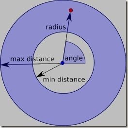
Figure 2 shows how a random point (red) is selected in the annulus around an existing point (blue). Two parameters determine the new point’s position: the angle (randomly chosen between 0 and 360 degrees), and the distance from the original point (randomly chosen between the minimum distance and twice the minimum distance). In pseudo code:
generateRandomPointAround(point, mindist)
{ //non-uniform, favours points closer to the inner ring, leads to denser packings
r1 = Random.nextDouble(); //random point between 0 and 1
r2 = Random.nextDouble();
//random radius between mindist and 2 * mindist
radius = mindist * (r1 + 1);
//random angle
angle = 2 * PI * r2;
//the new point is generated around the point (x, y)
newX = point.x + radius * cos(angle);
newY = point.y + radius * sin(angle);
return Point(newX, newY);
}
Figure 2 - Generating a new sample point.
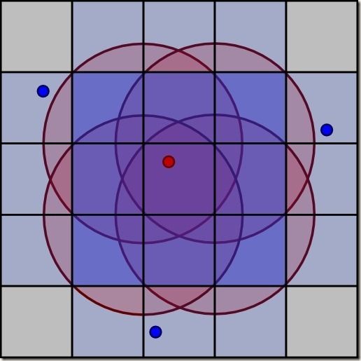
Before a newly generated point is admitted as a sample point, we have to check that no previously generated points are too close. Figure 3 shows a piece of the grid. The red dot is a potential new sample point. We have to check for existing points in the region contained by the red circles (they are the circles at the corners of the cell of the new point). The blue squares are cells that are partially or completely covered by a circle. We need only check these cells. However, to simplify the algorithm, we check all 25 cells.
Here is the pseudo code:
inNeighbourhood(grid, point, mindist, cellSize)
{
gridPoint = imageToGrid(point, cellSize)
//get the neighbourhood if the point in the grid
cellsAroundPoint = squareAroundPoint(grid, gridPoint, 5)
for every cell in cellsAroundPoint
if (cell != null)
if distance(cell, point) < mindist
return true
return false
}
Figure 3 - Checking the neighbourhood of a potential sample point.
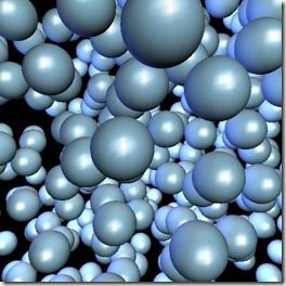
Figure 4 - Spheres placed at points in a Poisson disk sample of 3D space.
Implementation for 3D
The algorithm can easily be modified for 3D:
- Change all points to 3D points.
- Change the grid to a 3D grid. The neighbourhood of a point is now a cube of 125 cells around the cell of the point.
- Change the code to generate a new point to the following:
generateRandomPointAround(point, minDist)
{ //non-uniform, leads to denser packing.
r1 = Random.nextDouble(); //random point between 0 and 1
r2 = Random.nextDouble();
r3 = Random.nextDouble();
//random radius between mindist and 2* mindist
radius = mindist * (r1 + 1);
//random angle
angle1 = 2 * PI * r2;
angle2 = 2 * PI * r3;
//the new point is generated around the point (x, y, z)
newX = point.x + radius * cos(angle1) * sin(angle2);
newY = point.y + radius * sin(angle1) * sin(angle2);
newZ = point.z + radius * cos(angle2);
return Point(newX, newY, newZ);
}
Applications
Object Placement
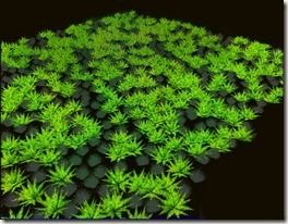
Placing objects at the positions of a Poisson disk sample set is the simplest way to use this algorithm in games (Figure 5). Ideally, the algorithm can be built into your level editing tool with features that allows the artist to select the region to fill, and the models to fill them with.
Figure 5 - An example with shrubs placed at Poisson disk sample points.
Figure 5 – An example with shrubs placed at Poisson disk sample points.
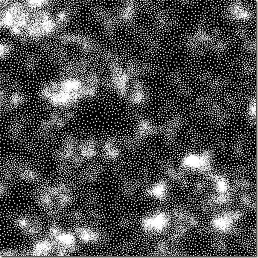
One important variation of a Poisson sample set is one where the minimum distance between points is not constant, but varies across the image. In this variation, we feed the algorithm a greyscale image, which is used to modulate the minimum distance between points.
To make this work, you need to modify the algorithm as follows:
- The grid must take a list of points.
- The cell size must be computed from the maximumthe radius can be.
- The neighbourhood function should iterate through all points in every cell of a point’s neighbourhood.
- Where a new point is generated, check the grey scale value of the image at that point, and calculate a minimum distance from the grey scale value:
min_dist = min_radius + grey * (max_radius - min_radius)
As an example, you can use Perlin noise to drive the minimum distance, giving you interesting clusters of objects (Figure 6). This method is especially useful for generating a field of plants.
Figure 6 - Poisson disk sample, where the minimum distance is driven by Perlin noise.
When using different radii as explained above, you might run into some problems. Take the following precautions:
- Ensure that your minimum radius is not too small. A very small radius might produce millions of points; a zero radius might prevent the algorithm from ever completing.
- Built in a bail-out feature in the algorithm, forcing it to end after a certain number of points have been reduced. Make it a function parameter, so that it can be modified according to the purpose. If you make a tool on top of this algorithm, also expose it to the user in the tool.
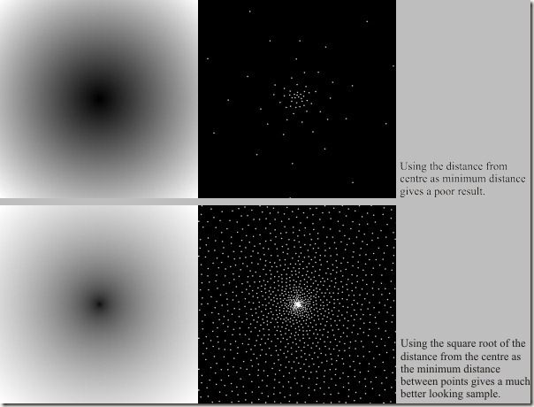
- Ensure that your maximum radius is not too big: if it is, no or very few points will be produced. This might seem obvious, but it can go wrong in a subtle way. Say, for example, you want to create a fall-off effect around a certain point. It would be natural to define your minimum distance array as follows:
min_dist[i, j] = dist((i, j), (x0, y0))
But because new points are generated at exactly this distance, many more points are excluded than expected, leading to a rather poor result. A better sample can be obtained by using the square root of the distance. (See Figure 7.)
Figure 7
In another situation, sections of large radii might be too close to other sections of large radii, so that no points are produced in sections of small radii (see Figure 8).
Figure 8 - The high radius is too great; some low radius regions are skipped.
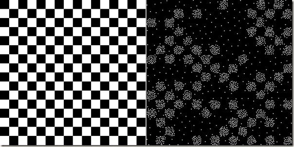
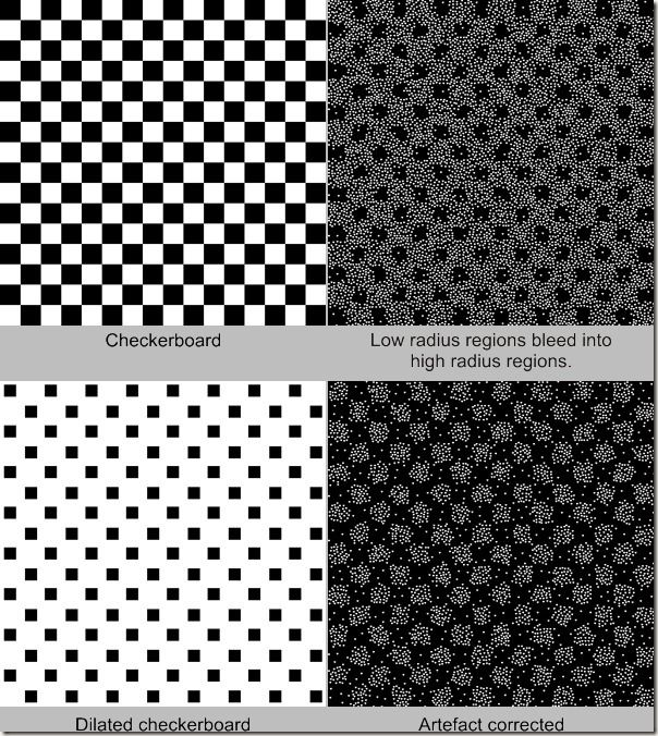
- For best results, your radius should vary smoothly across the rectangle. The algorithm respects sharp edges only ruggedly – see the checker board examples in Figure 9.
- Beware of the bleeding effect, as seen in Figure 9. You might want to run a dilation filter (use Photoshop or Gimp) on the radius grid before you do the sampling to compensate for this. Ideally the dilation should be a function of the minimum radius in a region, but in many cases you can used a fixed dilation.
Figure 9
Texture Generation
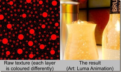
Poisson samples can also be used to generate certain textures. In Figure 10, the droplets on the bottle and glass have been created by combining three layers of Poisson disk sample points.
The modified algorithm creates three layers of points, each layer with a smaller minimum distance between points than the next. In every layer, the algorithm checks that there are no circles in the previous layers. To do this, the look-up grids for all generated layers are used in a final step to eliminate unwanted points.
The local minimum distance of a every sample point is stored, so that it can be used as a radius to draw a circle once all points have been found.
The raw texture is then further processed by clever artists through filters and shaders to produce the final result.
Figure 10.
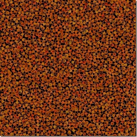
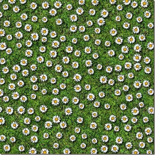
Poisson disk samples also form the basis of the procedural textures shown in Figure 11.
The first texture was produced by painting filled translucent circles for every Poisson sample point, for three separate samples. A different colour was used for every sample set, with small random variations.
The second texture was produced by painting circles for two sample sets; one with filled circles, the other with outlines only.
The third texture was created by painting daisies (randomly scaled and rotated) onto an existing grass texture.
Figure 11 - Procedural textures generated from Poisson disk samples.
Download
(Some of these links were added after the article was first published).
- You can download implementations in Java, Python, and Ruby for these algorithms fromhere.
- There is a C# implementation on Coderhaus, as well as a C# implementation by Renaud Bédard on The Instruction Limit.
- Kim Christiansen provides an
ActionScript 3 implementation on BigSource.
Resources
- Bridson R. Fast Poisson Disk Sampling in Arbitrary Dimensions.
The algorithm described in this article was taken from the paper above. - Dunbar, D.; Humphreys G. A Spatial Data Structure for Poisson-Disk Sample Generation.
Describes a fast algorithm for generating Poisson-Disk Sample sets in 2D. - Lagae, A.; Dutré P. A Comparison of Methods for Generating Poisson Disk Distributions.
An in-depth comparisson between different techniques for generating Poisson disk samples. - Talmor, D. Well-Spaced Points for Numerical Methods.
A comprehensive exploration of well-spaced points (including Poisson disk samples). Very mathematical!
