http://blog.csdn.net/pipisorry/article/details/43884027
机器学习Machine Learning - Andrew NG courses学习笔记
Logistic Regression逻辑回归
{逻辑回归是一种线性分类模型,而不是回归模型。也就是说,输入的因变量target y是离散值,如分类类别1,0等等,而不是连续型的数据。}
Classification分类(二分类)
0、1表示含义
denote with 0 is the negative class
denote with 1 is the positive class.
usually, use crosses to denote positive examples and O's to denote negative examples.
{Note:0 and 1 is somewhat arbitrary and it doesn't really matter.But often there is this intuition that the negative class is conveying the absence of something, like the absence of a malignant tumor.}
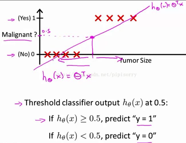
用线性规划来解决分类问题
Note: 实际上,分类器训练初始的分类面也是上图中一样的,与回归问题最大的不同还是训练阶段,回归问题用的是平方误差,而分类问题是其它特定误差。所以上图中的红线只是回归的拟合线,而回归的分类面实际是回归线上值为0.5对应的分类面!
looks like linear regression is actually doing something reasonable even though this is a classification task.
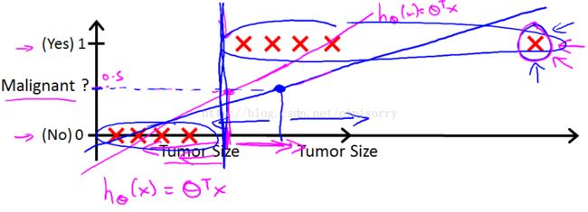
but if we got one more training example way out there on the right.
线性规划来解决分类问题的缺陷
加一个额外的数据(outliers)后线性规划就会出现不合理的结果(从magenta线到了blue线)。线性规划不能分类的原因主要是:outliers。平方误差由outliers控制,拉线。
另外线性规划还可能导致h(x) > 1 or < 0的问题。
所以将线性归划应用到分类问题上并不是个好idea。
为什么logistic regression能更好解决分类问题?
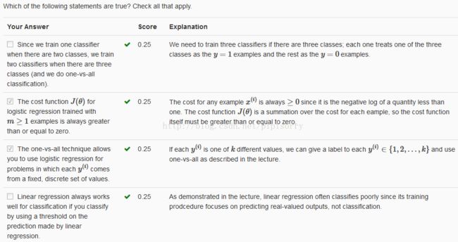
logistic regression will outperform linear regression since its cost function focuses on classification(假设数据是bern分布推导出的loss), not prediction. {lz:逻辑回归没有直线的拟合,它用分界面分割,分割错误会有很大的惩罚,所有更多的是关注于分类。如果有离群点且分割不好就会有很大惩罚(log函数作用),所以总体不会有太大误差。}
linear regression often classifies poorly since its training procedure focuses on predicting real-valued outputs, not classification.{线性规划是拟合出一条预测直线,所有数据离这根线越近越好。要是有离群点就会产生很大误差,可以看成是通过和拟合直线的距离最小化计算参数拟合直线。
而}
皮皮blog
Logistic回归的Cost Function代价函数
Hypothesis Representation假设表示式
{that is, what is the function we're going to use to represent our hypothesis where we have a classification problem.}
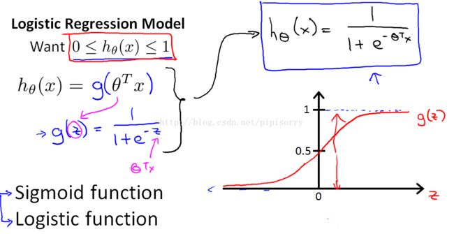
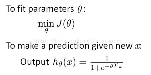
logistic regression假设表示就是在linear regression假设表示外面加一层sigmoid(logistic) function
logistic regression中logistic得名于logistic function。
为什么逻辑回归的假设hθ(x)要设计成这样?
1 预测的是离散的类label,或者预测位于[0,1]区间的后验概率分布。所以加上非线性函数(激活函数,如sigmod)对θ的线性函数进行变换。
2 sigmoid使预测位于[0,1],使用newton迭代求参时,Hessian矩阵正定,这样误差函数是参数的凸函数,从而具有唯一解。
3 求导方便;函数光滑什么的。广义线性?
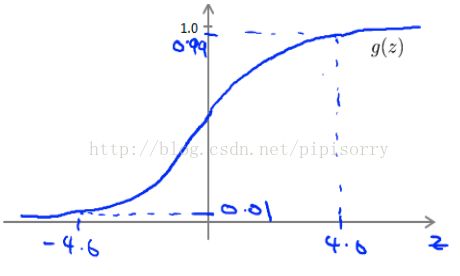
4 根据上图,可能是可以将0-1分类更好区分,如预测4.6时就基本接近1了,loss不会有什么惩罚。感觉就像是svm只关注支持向量一般(只是LR还以小概率关注了非支持向量)。
对某个输入x,hypothesis hθ(x)输出值的含义
此hypothesis代表 Y= 1 的概率。如示例中hypothesis告诉我们a patient with features X,y=1的概率为 0.7.
Decision Boundary决策边界
{sense of what the logistic regression hypothesis function is computing.}
既然h(x)代表the probability that Y=1,那通过什么predict y=1还是0值(通过θ'x来预测)。
假设θ0-2已知,一旦θ已知,就决定了决策边界,也就可以通过决策边界分割y的预测值。the decision boundary,the straight line, separates the region where the hypothesis predicts Y equals.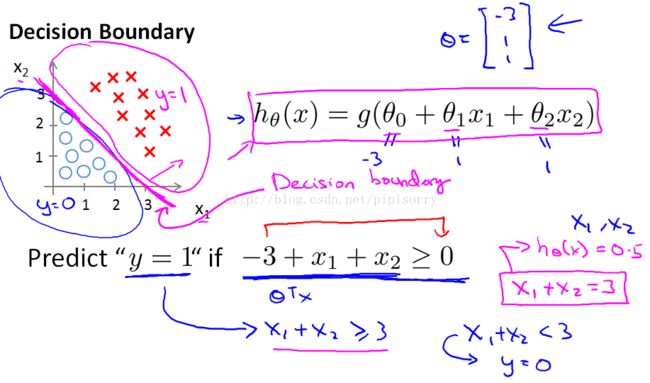
{决策边界和hypothesis、data set的关系: decision boundary是 hypothesis的性质和参数, 而不是data set的性质. The training set is not what we use to define decision boundary, but may be used to fit the parameters theta. But once you have the parameters theta, that is what defines the decision boundary.}
非线性决策边界
通过增加多项式项到feature中表示非线性决策边界。Earlier, when talking about polynomial regression or linear regression, we add extra higher order polynomial terms to the features.
So these higher order polynomial features you can get very complex decision boundaries.
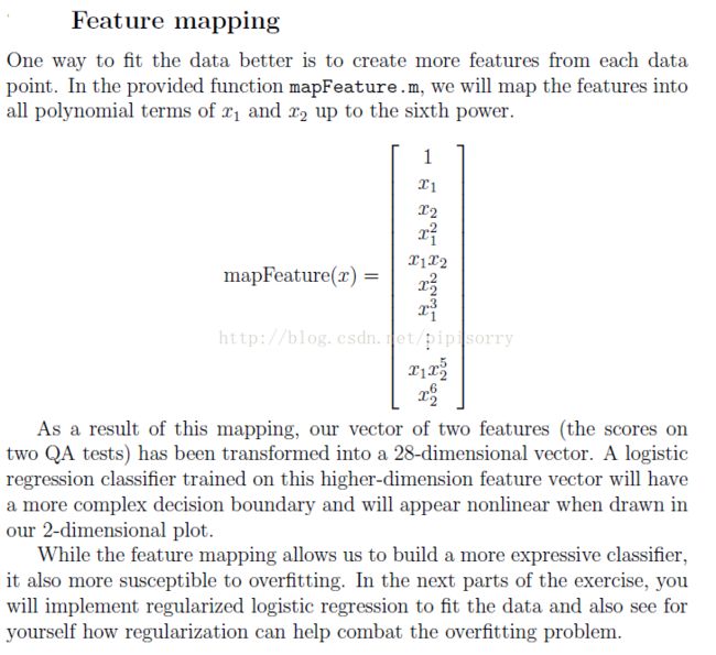
Feature mapping特征映射
function out = mapFeature(X1, X2)
% MAPFEATURE Feature mapping function to polynomial features
%
% MAPFEATURE(X1, X2) maps the two input features
% to quadratic features used in the regularization exercise.
%
% Returns a new feature array with more features, comprising of
% X1, X2, X1.^2, X2.^2, X1*X2, X1*X2.^2, etc..
%
% Inputs X1, X2 must be the same size
%
degree = 6;
out = ones(size(X1(:,1)));
for i = 1:degree
for j = 0:i
out(:, end+1) = (X1.^(i-j)).*(X2.^j);
end
end
end
Note: code to plot the non-linear boundary:(用contour图来画, x1, x2, z(即边界计算公式的值))
% Here is the grid range
u = linspace(-1, 1.5, 50);
v = linspace(-1, 1.5, 50);
z = zeros(length(u), length(v));
% Evaluate z = theta*x over the grid
for i = 1:length(u)
for j = 1:length(v)
z(i,j) = mapFeature(u(i), v(j))*theta;
end
end
z = z'; % important to transpose z before calling contour
% Plot z = 0
% Notice you need to specify the range [0, 0]
contour(u, v, z, [0, 0], 'LineWidth', 2)
逻辑回归的代价函数Cost Function(penalty function)!
convexity analysis凸分析
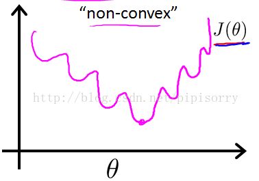
由于h(x)非线性(多项式features引起的?),导致参数θ的cost function J也是非线性(non-linear)的,图形也是非凸(non-convex)的,会有多个极小值点,用梯度下降方法不能保证得到全局最小值。
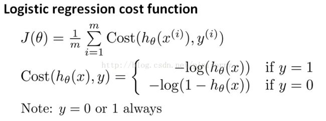
逻辑规划的代价函数
(for single training example只对J(θ)中的单个训练例子,而不是整个训练集)
从上可知,我们需要设计一个convex的cost func,这样就可以通过如gradient descent的方法保证得到全局最优值。
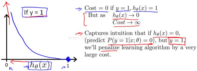
如果y=1而H(x)=0,我们就给这个学习算法一个非常非常大的接近infinity的惩罚。
为什么选择这个特殊的cost func?
因为逻辑回归假设数据是服从伯努力分布 Bern(x|u) = u^x * (1-u)^(1-x),即数据label要么是0要么是1。从而通过MLE推导得到这个loss func。并且这个loss func有一个很好convex性质。且从上面的图中看到,预测越偏离,惩罚越大。
简化逻辑回归的cost func
皮皮blog
梯度下降求解参数θ
{使用cost func对θ的梯度来更新θ。参数θ可以初始化为0或者随机初始化。}
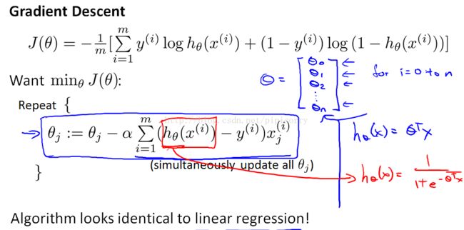
梯度下降Gradient Descent
Note:
1 即便logistic regression和linear regression Gradient descent的gradient descent更新规则表面上看起来一样,但其中的h(x)函数不同。
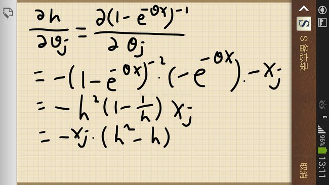
2 cost func对θ的梯度中偏导的推导:
3 我们可以使用类似线性规划的vectorized implementation来更新θ。
皮皮blog
Advanced Optimization高级优化方法
{be able to get logistic regression to run much more quickly than it's possible with gradient descent.And this will also let the algorithms scale much better to very large machine learning problems,such as if we had a very large number of features.}
an alternative view of what gradient descent is doing.(gradient descent is that we need to supply code to compute J of theta[technically you don't actually need code to compute the cost function J of theta(monitoring convergence)] and these derivatives, and then these get plugged into gradient descents, which can then try to minimize the function.)
最优化方法 - Gradient descent
其它最优化高级方法
if we only provide them a way to compute these two things[the cost function J of theta & the derivative terms], then these are different approaches to optimize the cost function.
Advantage1. You can think of these algorithms as having a clever inter-loop, called a line search algorithm that automatically tries out different values for the learning rate alpha and automatically picks a good learning rate alpha.so that it can even pick a different learning rate for every iteration.
Advantage2. These algorithms actually do more sophisticated things than just pick a good learning rate, and so they often end up converging much faster than gradient descent
使用octave解决最优化方法的一个简单Example:
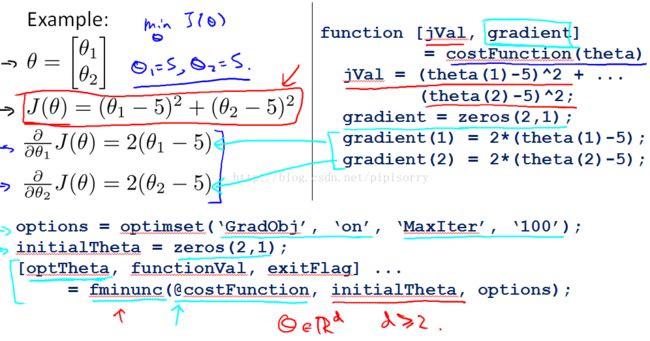
options:GradObj: So grant up on,this sets the gradient objective parameter to on.It just means you are indeed going to provide a gradient to this algorithm.(costFunction的第二个返回值)
fminunc: think it as just like gradient descent.But automatically choosing the learning rate alpha.
exit flag: let's you verify whether or not this algorithm thing has converged.
initialTheta: parameter vector of theta, must be in rd for d greater than or equal to 2.
`help fminunc` to read the documentation
use these optimization algorithms for linear regression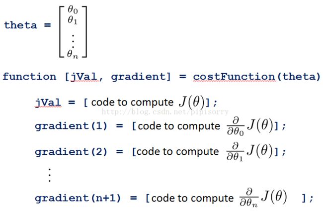
what you need to do,is write a function that returns the cost function and returns the gradient.
And so in order to apply this to logistic regression or even to linear regression.
Note: often quite typically whenever I have a large machine learning problem, I will use these algorithms instead of using gradient descent.
Note:
1. code to compute the sigmoid function:
g = 1.0 ./ (1 + exp(-z)); % Instructions: Compute the sigmoid of each value of z (z can be a matrix,vector or scalar).
2. code to compute the cost function:
J = -1 / m * (y' * log(sigmoid(X * theta)) + (1 - y)' * log(1 - sigmoid(X * theta)));
3. code to compute the gradient of the cost:
1> grad = (X' * (sigmoid(X * theta) - y)) / m; #vectorized,解释也可参见ex3.pdf - 1.3 Vectorizing Logistic Regression
2> for i=1:size(theta)
grad(i) = 1/m*(sigmoid(X*theta)-y)'*X(:,i);
end
4. use the logistic regression model to predict the probability that a student with score 45 on exam 1 and score 85 on exam 2 will be admitted.
prob = sigmoid([1 45 85] * theta);
5.Compute accuracy on our training set
p = sigmoid(X * theta) >= 0.5;
fprintf('Train Accuracy: %f\n', mean(double(p == y)) * 100);
皮皮blog
Multiclass Classification多类分类
{variable Y may take on for value zero, one, two and three.Not just zero and one.}
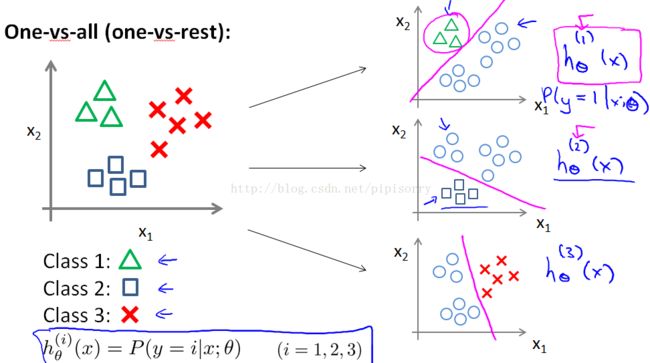
one-versus-all(one versus rest)classification
take a training set, and, turn this into three separate binary classification problems.essentially create a new, sort of fake training set.where classes 2 and 3 get assigned to the negative class and class 1 gets assigned to the positive class.
将多分类转化成二分类,h(x)的值就是p(y = 1)就是positive class的概率。{p(y = 0)是无意义的}。每个分类器对应预测一个分类。
for this first classifier with learning to by the triangle.So it's thinking of the triangles as a positive class.So, X superscript one is essentially trying to estimate what is the probability that the Y is equal to one, given X and parametrized by theta.
training训练:
Note:想起一个问题,会不会存在不确定区域?由于逻辑规划并非线性判别,应该不存在不确定区域,只要哪个概率大,就属于哪个类了,并不会出现不能分类的情况。
Code for one-vs-all algorithm in handwriting recognition:
Note:
{make sure that your regularized logistic regression implementation is vectorized.}
load data:
The .mat format means that that the data has been saved in a native Octave/Matlab matrix format, instead of a text (ASCII) format like a csv-file. These matrices can be read directly into your program by using the load command. After loading, matrices of the correct dimensions and values will appear in your program's memory. The matrix will already be named, so you do not need to assign names to them.
% Load saved matrices from file
load('ex3data1.mat');
% The matrices X and y will now be in your Octave environment
oneVsAll algorithm:
all_theta = zeros(num_labels, n + 1);
% Add ones to the X data matrix
X = [ones(m, 1) X];
% Instructions:
% Hint: You can use y == c to obtain a vector of 1's and 0's that tell use whether the ground truth is true/false for this class.
%
% Note: For this assignment, we recommend using fmincg to optimize the cost function. It is okay to use a for-loop (for c = 1:num_labels) to loop over the different classes.
% fmincg works similarly to fminunc, but is more efficient when we are dealing with large number of parameters.
%
initial_theta = zeros(n + 1, 1);
options = optimset('GradObj', 'on', 'MaxIter', 50);
for c = 1:num_labels,
all_theta(c, :) = (fmincg (@(t)(lrCostFunction(t, X, (y == c), lambda)), initial_theta, options))';
end
predictOneVsAll
%hint: If your examples are in rows, then, you can use max(A, [], 2) to obtain the max for each row.
[max_in_rows,c] = (max(X * all_theta', [], 2));
p = c;
皮皮blog
Review复习
from:http://blog.csdn.net/pipisorry/article/details/43884027
ref:Logistic回归深入理解指南《Guide to an in-depth understanding of logistic regression》by Kevin Markham
Logic of Logistic Regression
Logistic Regression
