【Machine Learning】3.多元线性回归

本文包括多元线性回归代价计算和梯度下降的理论部分和实践部分，并留有课后作业

一般的回归步骤：问题描述->导入数据集并检查分析数据意义和特征->repeat{梯度计算->梯度下降->代价计算（评估值的优劣）}->预测

1.导入

import copy, math
import numpy as np
import matplotlib.pyplot as plt
plt.style.use('./deeplearning.mplstyle')
np.set_printoptions(precision=2)  # reduced display precision（精度） on numpy arrays

2.问题描述

2.1 Matrix X containing our examples

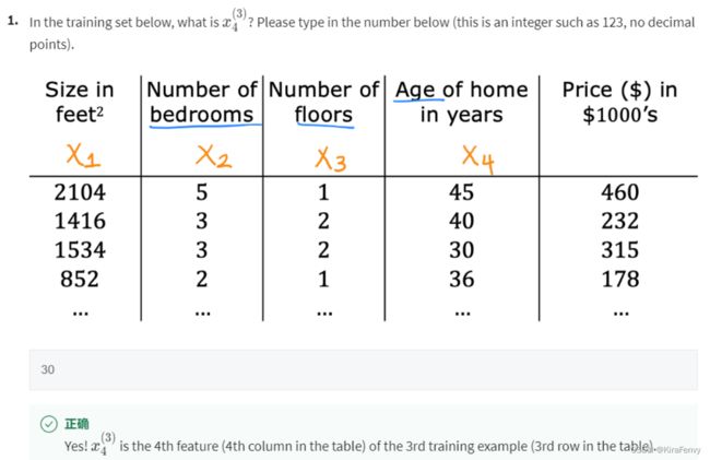
Similar to the table above, examples are stored in a NumPy matrix X_train. Each row of the matrix represents one example. When you have $m$ training examples ( $m$ is three in our example), and there are $n$ features (four in our example), $\mathbf{X}$ is a matrix with dimensions ($m$, $n$) (m rows, n columns). 每一行代表一个例子，每一列是一个特征，例子编号右上角，特征编号右下角

$$\mathbf{X}=\left(\begin{array}{cccc}{x}_0^{(0)}& x_1^{(0)}& \cdots & x_{n-1}^{(0)}\\ x_0^{(1)}& x_1^{(1)}& \cdots & x_{n-1}^{(1)}\\ \cdots & & & \\ x_0^{(m-1)}& x_1^{(m-1)}& \cdots & x_{n-1}^{(m-1)}\end{array}\right)$$
notation:

• ${\mathbf{x}}^{(i)}$ is vector containing example i. ${\mathbf{x}}^{(i)}=(x_0^{(i)},x_1^{(i)},\cdots ,x_{n-1}^{(i)})$
• $x_j^{(i)}$ is element j in example i. The superscript in parenthesis indicates the example number while the subscript represents an element. 上标表示示例编号，而下标表示元素。

创建数据或者导入训练集：

X_train = np.array([[2104, 5, 1, 45], [1416, 3, 2, 40], [852, 2, 1, 35]])
y_train = np.array([460, 232, 178])

# load the dataset
x_train, y_train = load_data()

查看一下数据类型和头5条数据，思考这些数据的意义（如x代表价格单位元，y代表人口，单位万人）

# print x_train
print("Type of x_train:",type(x_train))
print("First five elements of x_train are:\n", x_train[:5]) 

# print y_train
print("Type of y_train:",type(y_train))
print("First five elements of y_train are:\n", y_train[:5]) 

检查一下数据维度

print ('The shape of x_train is:', x_train.shape)
print ('The shape of y_train is: ', y_train.shape)
print ('Number of training examples (m):', len(x_train))

可以可视化数据

# Create a scatter plot of the data. To change the markers to red "x",
# we used the 'marker' and 'c' parameters
plt.scatter(x_train, y_train, marker='x', c='r') 

# Set the title
plt.title("Profits vs. Population per city")
# Set the y-axis label
plt.ylabel('Profit in $10,000')
# Set the x-axis label
plt.xlabel('Population of City in 10,000s')
plt.show()

2.2 Parameter vector w, b

• $\mathbf{w}$ is a vector with $n$ elements.
  • Each element contains the parameter associated with one feature.
  • notionally, we draw this as a column vector 列向量

$$\mathbf{w}=\left(\begin{array}{c}{w}_0\\ w_1\\ \cdots \\ w_{n-1}\end{array}\right)$$

• $b$ is a scalar parameter.

b_init = 785.1811367994083
w_init = np.array([ 0.39133535, 18.75376741, -53.36032453, -26.42131618])

3 多元的模型预测方法

The model’s prediction with multiple variables is given by the linear model:

$$f_{\mathbf{w},b}(\mathbf{x})=w_0{x}_0+w_1{x}_1+...+w_{n-1}{x}_{n-1}+b\text{\hspace{1em}(1)}$$
向量表示为:
$$f_{\mathbf{w},b}(\mathbf{x})=\mathbf{w}\cdot \mathbf{x}+b\text{\hspace{1em}(2)}$$
where $\cdot$ is a vector dot product点积

To demonstrate the dot product, we will implement prediction using (1) and (2).

3.1 Single Prediction element by element

Our previous prediction multiplied one feature value by one parameter and added a bias parameter. A direct extension of our previous implementation of prediction to multiple features would be to implement (1) above using loop over each element, performing the multiply with its parameter and then adding the bias parameter at the end.

def predict_single_loop(x, w, b): 
    """
    single predict using linear regression
    
    Args:
      x (ndarray): Shape (n,) example with multiple features
      w (ndarray): Shape (n,) model parameters    
      b (scalar):  model parameter     
      
    Returns:
      p (scalar):  prediction
    """
    n = x.shape[0]
    p = 0
    for i in range(n):
        p_i = x[i] * w[i]  
        p = p + p_i         
    p = p + b                
    return p

3.2 Single Prediction, vector

使用点积来加速上述实现

def predict(x, w, b): 
    """
    single predict using linear regression
    Args:
      x (ndarray): Shape (n,) example with multiple features
      w (ndarray): Shape (n,) model parameters   
      b (scalar):             model parameter 
      
    Returns:
      p (scalar):  prediction
    """
    p = np.dot(x, w) + b     
    return p    

4 多元代价计算

The equation for the cost function with multiple variables $J(\mathbf{w},b)$ is:
$$J(\mathbf{w},b)=\frac{1}{2m}\sum _{i=0}^{m-1}(f_{\mathbf{w},b}({\mathbf{x}}^{(i)})-y^{(i)}{)}^2\text{\hspace{1em}(3)}$$
where:
$$f_{\mathbf{w},b}({\mathbf{x}}^{(i)})=\mathbf{w}\cdot {\mathbf{x}}^{(i)}+b\text{\hspace{1em}(4)}$$

In contrast to previous labs, $\mathbf{w}$ and ${\mathbf{x}}^{(i)}$ are vectors rather than scalars 标量 supporting multiple features.

def compute_cost(X, y, w, b): 
    """
    compute cost
    Args:
      X (ndarray (m,n)): Data, m examples with n features
      y (ndarray (m,)) : target values
      w (ndarray (n,)) : model parameters  
      b (scalar)       : model parameter
      
    Returns:
      cost (scalar): cost
    """
    m = X.shape[0]
    cost = 0.0
    for i in range(m):                                
        f_wb_i = np.dot(X[i], w) + b           #(n,)(n,) = scalar (see np.dot)
        cost = cost + (f_wb_i - y[i])**2       #scalar
    cost = cost / (2 * m)                      #scalar    
    return cost

# Compute and display cost using our pre-chosen optimal parameters. 
cost = compute_cost(X_train, y_train, w_init, b_init)
print(f'Cost at optimal w : {cost}')

5 多元梯度下降

Gradient descent for multiple variables:

$$\begin{array}{rlr}\text{repeat}& \text{ until convergence:}\{& \\ & w_j=w_j-\alpha \frac{\partial J(\mathbf{w},b)}{\partial w_j}& \text{for j = 0..n-1}\\ & b=b-\alpha \frac{\partial J(\mathbf{w},b)}{\partial b}& \\ \}& & \end{array}\text{\hspace{1em}(5)}$$

where, n is the number of features n为特征个数, parameters $w_j$, $b$, are updated simultaneously and where

$$\begin{array}{rl}\frac{\partial J(\mathbf{w},b)}{\partial w_j}& =\frac{1}{m}\sum _{i=0}^{m-1}(f_{\mathbf{w},b}({\mathbf{x}}^{(i)})-y^{(i)})x_j^{(i)}\\ \frac{\partial J(\mathbf{w},b)}{\partial b}& =\frac{1}{m}\sum _{i=0}^{m-1}(f_{\mathbf{w},b}({\mathbf{x}}^{(i)})-y^{(i)})\end{array}\text{\hspace{1em}(6)(7)}$$

• m is the number of training examples in the data set 训练集例子个数

• $f_{\mathbf{w},b}({\mathbf{x}}^{(i)})$ is the model’s prediction, while $y^{(i)}$ is the target value

5.1 计算梯度

An implementation for calculating the equations (6) and (7) is below. There are many ways to implement this. In this version, there is an 一个循环计算梯度的方法：

• Return the total gradient update from all the examples
  $$\frac{\partial J(w,b)}{\partial b}=\frac{1}{m}\sum _{i=0}^{m-1}{\frac{\partial J(w,b)}{\partial b}}^{(i)}$$

  $$\frac{\partial J(w,b)}{\partial w}=\frac{1}{m}\sum _{i=0}^{m-1}{\frac{\partial J(w,b)}{\partial w}}^{(i)}$$

  • Here, $m$ is the number of training examples and $\sum$ is the summation operator

• outer loop over all m examples.
  • $\frac{\partial J(\mathbf{w},b)}{\partial b}$ for the example can be computed directly and accumulated
  • in a second loop over all n features:
    • $\frac{\partial J(\mathbf{w},b)}{\partial w_j}$ is computed for each $w_j$.

def compute_gradient(X, y, w, b): 
    """
    Computes the gradient for linear regression 
    Args:
      X (ndarray (m,n)): Data, m examples with n features
      y (ndarray (m,)) : target values
      w (ndarray (n,)) : model parameters  
      b (scalar)       : model parameter
      
    Returns:
      dj_dw (ndarray (n,)): The gradient of the cost w.r.t. the parameters w. 
      dj_db (scalar):       The gradient of the cost w.r.t. the parameter b. 
    """
    m,n = X.shape           #(number of examples, number of features)
    dj_dw = np.zeros((n,))
    dj_db = 0.

    for i in range(m):                             
        err = (np.dot(X[i], w) + b) - y[i]   
        for j in range(n):                         
            dj_dw[j] = dj_dw[j] + err * X[i, j]    
        dj_db = dj_db + err                        
    dj_dw = dj_dw / m                                
    dj_db = dj_db / m                                
        
    return dj_db, dj_dw

5.2 梯度下降

注意在梯度下降的函数当中，调用了前面的代价计算函数和梯度计算函数，一般先算出梯度，然后用梯度进行梯度下降后面算出代价进行评估（只是因为我们需要审查代价的history评估整个回归过程），最后返回若干次迭代后的w和b为最优值

The routine below implements equation (5) above.
$$\begin{array}{rlr}\text{repeat}& \text{ until convergence:}\{& \\ & w_j=w_j-\alpha \frac{\partial J(\mathbf{w},b)}{\partial w_j}& \text{for j = 0..n-1}\\ & b=b-\alpha \frac{\partial J(\mathbf{w},b)}{\partial b}& \\ \}& & \end{array}\text{\hspace{1em}(5)}$$

def gradient_descent(X, y, w_in, b_in, cost_function, gradient_function, alpha, num_iters): 
    """
    Performs batch gradient descent to learn theta. Updates theta by taking 
    num_iters gradient steps with learning rate alpha
    
    Args:
      X (ndarray (m,n))   : Data, m examples with n features
      y (ndarray (m,))    : target values
      w_in (ndarray (n,)) : initial model parameters  
      b_in (scalar)       : initial model parameter
      cost_function       : function to compute cost
      gradient_function   : function to compute the gradient
      alpha (float)       : Learning rate
      num_iters (int)     : number of iterations to run gradient descent
      
    Returns:
      w (ndarray (n,)) : Updated values of parameters 
      b (scalar)       : Updated value of parameter 
      """
    
    # An array to store cost J and w's at each iteration primarily for graphing later
    J_history = []
    w = copy.deepcopy(w_in)  #avoid modifying global w within function
    b = b_in
    
    for i in range(num_iters):

        # Calculate the gradient and update the parameters
        dj_db,dj_dw = gradient_function(X, y, w, b)   ##None

        # Update Parameters using w, b, alpha and gradient
        w = w - alpha * dj_dw               ##None
        b = b - alpha * dj_db               ##None
      
        # Save cost J at each iteration
        if i<100000:      # prevent resource exhaustion 
            J_history.append( cost_function(X, y, w, b))

        # Print cost every at intervals 10 times or as many iterations if < 10
        if i% math.ceil(num_iters / 10) == 0:
            print(f"Iteration {i:4d}: Cost {J_history[-1]:8.2f}   ")
        
    return w, b, J_history #return final w,b and J history for graphing

这里返回w和b，最后就可以用算出来的w和b预测了

# initialize parameters
initial_w = np.zeros_like(w_init)
initial_b = 0.
# some gradient descent settings
iterations = 1000
alpha = 5.0e-7
# run gradient descent 
w_final, b_final, J_hist = gradient_descent(X_train, y_train, initial_w, initial_b,
                                                    compute_cost, compute_gradient, 
                                                    alpha, iterations)
print(f"b,w found by gradient descent: {b_final:0.2f},{w_final} ")
m,_ = X_train.shape
for i in range(m):
    print(f"prediction: {np.dot(X_train[i], w_final) + b_final:0.2f}, target value: {y_train[i]}")

6 课后习题

1. 考查表示方法
   

2. 向量化的优点包括使代码更简洁、便于并行计算，加快速度
   

3. 学习率double，梯度收敛速度不一定double，因为可能导致无法收敛到最优值
   

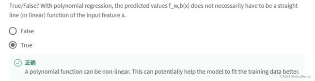
4. 多项式回归是非线性的，不一定要有b也能拟合