可解释机器学习
重点 (Top highlight)
In this post, we will get the idea of Shapley value, try to understand why the order of features matter, how to move from Shapley value to SHAP, the story of Observational and Interventional Conditional Distribution when filling absent features, should we use train set or test set for explaining the model and so forth.
在这篇文章中,我们将获得Shapley值的概念,尝试理解为什么特征顺序很重要,如何从Shapley值转换为SHAP,以及在填充缺失特征时如何观察和介入条件分布的故事,是否应该使用训练集或用于解释模型的测试集等。
1. Shapley值 (1. Shapley value)
SHAP is based on Shapley value, so we need to know what is the Shapley value first.
SHAP基于Shapley值,因此我们首先需要知道Shapley值是什么。
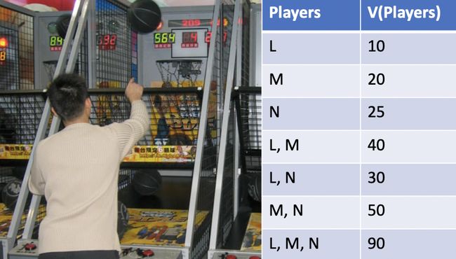
Let’s say we have 3 players namely L, M, N going for a basketball game with machines. If L plays alone, he can earn 10 points. For M’s and N’s, the numbers are 20 and 25 points, respectively. If L and M play together, somehow they know how to collaborate and end up with 40 points. However, when L and N team up, they get only 30 points. The details are shown in the following table, where v(S) is the total contribution that members in S can get by cooperation.
假设我们有3名球员,分别是L,M,N,他们正在用机器进行篮球比赛。 如果L一个人玩,他可以获得10分。 对于M和N,数字分别为20和25点。 如果L和M一起比赛,他们将以某种方式知道如何合作并最终获得40分。 但是,当L和N组队时,他们只得到30分。 详细情况如下表所示,其中V(S)是总贡献S中的成员可以通过合作进入。
Contribution of each coalition. 每个联盟的贡献。How can we find the contribution of each player in the team with the information above? Which player is the best among the three?
通过上面的信息,我们如何找到团队中每个球员的贡献? 三者中哪一个是最好的?
The contribution of a player, L for example, can be calculated by the difference that L brings up to the final score. In other words, we consider the difference when having L in the game compared to when he is not. To further break down, when L joins in, L may play alone, or he can play together with other members. Thus, intuitively, the final contribution of L should be a form of the average of all the cases:
玩家的贡献,例如L,可以通过L达到最终得分的差来计算。 换句话说,我们考虑在游戏中拥有L时与没有L时的差异。 为了进一步分解,当L加入时,L可以单独玩,也可以与其他成员一起玩。 因此,从直觉上讲,L的最终贡献应该是所有情况的平均值的形式:
Mathematically, assume we have a set N containing all the players, S is a coalition (subset) of players. The contribution of player i (φi ) as we suggested can be rewritten as:
在数学上,假设我们有一个包含所有参与者的集合N , S是参与者的联盟(子集)。 参与者i(φI)为我们提出的贡献可以被改写为:
It comes close to the formula that was proposed in the Shapley value.
它与Shapley值中提出的公式非常接近。
“The Shapley value is a solution concept in cooperative game theory. It was named in honor of Lloyd Shapley, who introduced it in 1951 and won the Nobel Prize in Economics for it in 2012” — Wiki
Shapley值是合作博弈论中的解决方案概念。 它以纪念劳埃德·沙普利 ( Lloyd Shapley )的名字命名,后者于1951年推出了该模型,并于2012年获得了诺贝尔经济学奖。” — Wiki
Lloyd Shapley wanted to calculate the contribution of each player in a coalition game. The idea is that considering all possible different permutations, we get the contribution of a player in each game by using marginal contribution, then taking the average of these contributions to get the final contribution of that player [11]. The thing that we’re missing in the Shapley value’s formula, is the ordering part.
劳埃德·沙普利(Lloyd Shapley)希望计算联盟游戏中每个玩家的贡献。 这个想法是考虑所有可能的不同排列,我们通过使用边际贡献来获得每个游戏中玩家的贡献,然后取这些贡献的平均值以获得该玩家的最终贡献[11]。 Shapley值公式中缺少的是排序部分。
Shapley value’s formula. The ordering part is in the blue box. Shapley值的公式。 订购部分在蓝色框中。Where|N|! in the denominator indicates all possible permutations. In the numerator, |S|!(|N| — |S| — 1)! depicts that the term (v(S⋃{i}) — v(x)) will appear|S|!(|N| — |S| — 1)! times in total |N|! permutations.
| N |! 分母中的表示所有可能的排列。 在分子中, | S |!(| N | — | S | — 1)! 描绘了(v(S⋃{i})— v(x))项将出现| S |!(| N | — | S | — 1)! 总次数| N |! 排列。
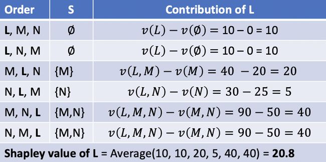
Get back to the beginning example, we get the Shapley value for L as below.
回到开始的示例,我们得到L的Shapley值,如下所示。
|S|!(|N| — |S| — 1)! of these terms will be 2 in the Shapley value’s formula. | S |!(| N | — | S | — 1)的值! Shapley值公式中的这些项中的2将为2。2.为什么功能顺序很重要? (2. Why the order of features matter?)
Why Shapley values take into account the order?
为什么Shapley值会考虑顺序?
In some cases, the order plays an essential role when there are overlaps amongst the features.
在某些情况下,订单起着至关重要的作用 当特征之间有重叠时 。
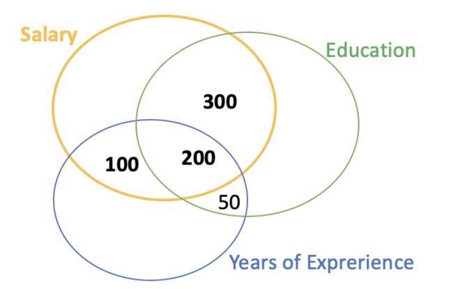
For example, when the first feature comes in, it contributes significantly to the model’s performance. The second feature joins later on, and because it has a big overlap with the first feature, the new feature does not add much “new knowledge” to our model. It’s the other way around when we reverse the order. The picture below indicates the scenario, with two features namely Education and Years of Experience to predict Salary.
例如,当第一个功能进入时,它将对模型的性能做出重大贡献。 第二个功能稍后会加入,由于它与第一个功能有很大的重叠,因此新功能不会为我们的模型增加太多“新知识”。 当我们颠倒顺序时,这是另一回事。 下图显示了这种情况,具有两个功能,即“教育”和“工作年限”以预测薪资。
If Education is added first, it will contribute to the model 500 points, then the YearsOfExperience comes in and only adds 100 more. Reversely, when the YearsOfExperience is added first, it can give 300 points to the model. After that, Education comes and contributes 300 more. Shapley values consider both of the cases to compute the feature importance (200 for YearsOfExperience, and 400 for Education). That’s why the order is taken into account when calculating the Shaley values. 如果首先添加教育,它将为模型贡献500分,然后进入YearsOfExperience,而仅增加100分。 相反,当首先添加YearsOfExperience时,可以为模型提供300分。 之后,教育来了,又贡献了300多。 Shapley值会考虑这两种情况,以计算功能的重要性(“ YearsOfExperience”为200,“教育”为400)。 这就是为什么在计算Shaley值时要考虑顺序的原因。Sum up so far: The main idea of Shapley Values is to get the Marginal contributions of a feature in all different orders, then take the average. In other words, we consider the difference in the performance of our model with and without the feature, in all possible ordering.
到目前为止,总结: Shapley值的主要思想是获取特征在所有不同顺序中的边际贡献,然后取平均值。 换句话说,在所有可能的顺序中,我们都会考虑具有和不具有功能的模型的性能差异。
3. SHAP(希普利添加剂) (3. SHAP (SHapley Additive exPlanations))
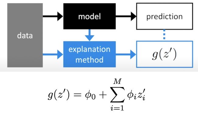
SHAP (SHapley Additive exPlanations), first introduced by Scott Lundberg and Su-In Lee in 2017, is a game-theoretic approach to explain the output of any machine learning model. It employs the classic Shapley values from game theory to explain the model to the individual data point level [12].
SHAP(SHapley Additive exPlanations)由Scott Lundberg和Su-In Lee于2017年首次提出,它是一种博弈论方法,可以解释任何机器学习模型的输出。 它利用博弈论中的经典Shapley值将模型解释为单个数据点级别[12]。
3.1。 SHAP论文的主要贡献[1,2,3] (3.1. Main contributions of SHAP’s papers [1,2,3])
The authors defined a new class of additive feature importance methods. The new view shows an interesting connection between six other methods such as LIME, DeepLIFT.
作者定义了一类新的加性特征重要性方法。 新视图显示了六个其他方法(例如LIME和DeepLIFT)之间的有趣联系。
- SHAP explanation method computes Shapley values from coalitional game theory. The authors introduced three Theoretical Properties for SHAP (Local accuracy, Missingness, and Consistency)[1], which are familiar to the four properties of classical Shapley value (Efficiency, Symmetry, Dummy, and Additivity)[11]. SHAP解释方法根据联盟博弈理论计算Shapley值。 作者介绍了SHAP的三个理论属性(局部精度,缺失和一致性)[1],这是经典Shapley值的四个属性(效率,对称性,虚拟和可加性)[11]。
The papers proposed a model-agnostic method named KernelSHAP, and properly the most well-known one for tree-based models (e.g., LightGBM, XGboost, CatBoost) named TreeExplainer.
论文提出了一种与模型无关的方法,称为KernelSHAP ,并且是树型模型(例如LightGBM,XGboost,CatBoost)最知名的方法,即TreeExplainer。
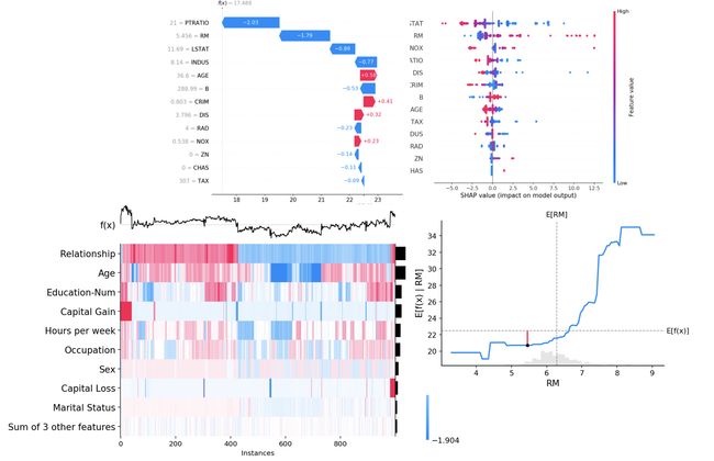
Not only can SHAP explain to the individual level, it also gives some out-of-the-box techniques to combine the explanations into global explanations such as feature importance, feature dependence, interactions, clustering, and summary plot.
SHAP不仅可以对个人进行解释,而且还提供了一些开箱即用的技术,可以将解释合并为全局解释,例如特征重要性,特征依赖性,交互作用,聚类和摘要图。
We will go more details on SHAP in the next section.
我们将在下一节中详细介绍SHAP。
3.2。 为什么精确的Shapley值昂贵? (3.2. Why are exact Shapley values expensive?)
The first thing that SHAP needs to deal with, is how to compute the Shapely values efficiently.
SHAP需要处理的第一件事是如何有效地计算Shapely值。
In fact, the exact computation of Shapley values is extremely expensive. For F features, we have 2^F subsets S. To compute the exact Shapley values, we have to re-train a new model on the features in each S. It’s obviously a lot of work and impractical in the real world.
实际上,精确计算Shapley值非常昂贵。 对于F个要素,我们有2 ^ F个子集S。要计算确切的Shapley值,我们必须对每个S中的要素重新训练一个新模型。在现实世界中,这显然是很多工作且不切实际。
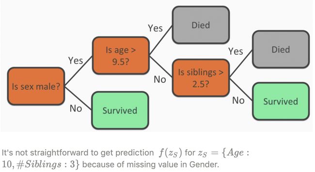
You may argue that why we need to re-train a lot of models, instead of using the one that is already trained with all the features. Let’s call S is the set of features we have the values, and C is the set of features that we don’t. Assume we have a decision tree f on Titanic data with three features (Gender, Age, and #Siblings), S = {Age, #Siblings}, and the missing feature set C = {Gender} (figure below). How can get the prediction f(z_S), with z_S = {Age: 10, #Siblings: 3} (i.e., missing Gender’s value).
您可能会争辩说,为什么我们需要重新训练很多模型,而不是使用已经使用所有功能进行训练的模型。 我们称S为具有值的要素集,而C为没有值的要素集。 假设我们在泰坦尼克号数据上有一个决策树f ,具有三个特征( Gender , Age和#Siblings ), S = { Age , #Siblings }和缺少的特征集C = { Gender }(下图)。 如何获得预测f(z_S) , z_S = { 年龄 :10,# 兄弟姐妹 :3}(即,缺少性别值)。
From a given model f, it is not so immediately clear how to get the prediction f(z_S) when having a set of missing values in C. Thus, in general, we need 2^F models to get the exact Shapley values which make the computation of Shapley values expensive.
从给定的模型f中 ,当在C中具有一组缺失值时,还不是很清楚如何获得预测f(z_S) 。 因此,一般而言,我们需要2 ^ F模型来获取精确的Shapley值,这使得Shapley值的计算变得昂贵。
3.3。 SHAP如何近似于Shapley值? (3.3. How does SHAP approximate Shapley values?)
SHAP approximates the Shapley values of a conditional expectation function of the original model [1]. More specifically, it approximates the function f(z_S) by a conditional expectation E[f(z_S, z_C)|z_S] (Eq. 9 in the SHAP paper [1]).
SHAP近似原始模型的条件期望函数的Shapley值[1]。 更具体地说,它通过条件期望E [f(z_S,z_C)| z_S]来近似函数f(z_S) (在SHAP论文[1]中, 方程9 )。
Equations in the SHAP paper [1] SHAP论文中的方程[1]From the Eq. 9 (Conditional Expectation), we use the Law of Total Expectation with z_C and then assume that the features are independent to get the approximation in Eq. 11 (Marginal Expectation) as the following.
从等式 9 (有条件期望),我们将总期望定律与z_C一起使用 ,然后假定特征是独立的,以得到等式中的近似值。 11 (边际期望)如下。
Let’s get back to the Titanic example. We need to get the prediction f(z_S), with z_S = {Age: 10, #Siblings: 3}. From Eq. 11, f(z_S) can be approximated by E_{z_C}[f(z)] = E_{Gender}[f(Age:10, #Siblings:3, Gender: missing)].
让我们回到泰坦尼克号的例子。 我们需要获得预测f(z_S) ,其中z_S = {年龄:10,#Siblings:3} 。 从等式 如图11所示 ,可以通过E_ {z_C} [f(z)] = E_ {性别} [f(年龄:10,#Siblings:3,性别:缺失)]来近似f(z_S) 。
To calculate E_{z_C}[f(z)], with tabular data, absent features can be randomly drawn from background data (e.g., the rest of the dataset). For images, we can take the average of surrounding pixels/superpixels, or even simply just assign it to zeros.
为了使用表格数据计算E_ {z_C} [f(z)] ,可以从背景数据(例如,数据集的其余部分)中随机绘制缺少的特征。 对于图像,我们可以取周围像素/超像素的平均值,甚至只是将其分配为零即可。
So, after filling missing values, we can calculate Marginal Expectation E_{z_C}[f(z)] to get an approximation for f(z_S).
因此,在填充缺失值之后,我们可以计算边际期望E_ {z_C} [f(z)]以获得f(z_S)的近似值。
If the model is linear, from the Eq.11, we can further simplify it to Eq.12. Recall that E[f(x)] = f(E[x]) when f(x) is a linear model.
如果模型是线性的,则从等式11可以进一步简化为等式12。 回想一下,当f(x)是线性模型时, E [f(x)] = f(E [x]) 。
Sum up so far: SHAP makes an assumption about feature independence. It approximates Shapley values by using Marginal distribution to impute absent features.
到目前为止的总结: SHAP对功能独立性进行了假设。 它通过使用边际分布估算缺少的特征来近似Shapley值。
4.我们应该如何填补缺失的特征? (4. How should we fill absent features?)
This is an interesting topic related to Interpretability and Causality. First of all, we need to get an idea of the Observational and Interventional Conditional Distribution.
这是一个与可解释性和因果关系有关的有趣话题。 首先,我们需要了解观察和介入条件分布。
4.1。 观察与介入条件分布 (4.1. Observational vs. Interventional Conditional Distribution)
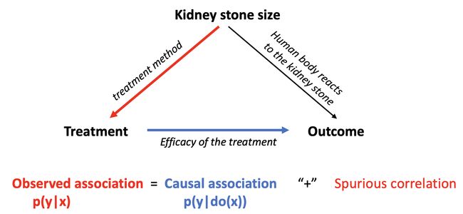
I borrow an example from [14] which is shown in the following picture. Basically, we have 3 factors namely Kidney stone size, Treatment, and Outcome. The red line indicates that a certain size of kidney stones will affect which treatment to be assigned. The blue line presents a direct relationship between treatments and outcomes.
我从[14]中借用了一个示例,如下图所示。 基本上,我们有3个因素,即肾结石大小,治疗和结果 。 红线表示一定尺寸的肾结石将影响应分配的治疗方法。 蓝线表示治疗与结果之间的直接关系。
Given x is a medical treatment and y is the outcome, p(y|x) is what we observed from x to infer the value of y, while p(y|do(x)) indicates how intervention on x effects y in causal Inference perspective. 给定x是药物治疗,y是结果,则p(y | x)是我们从x观察到的推论y的值,而p(y | do(x))表示对x进行干预如何在因果关系中影响y推理角度。When observing how the treatment is associated with positive outcomes (p(y|x)), we actually measure two separate components: the actual causal relationship (written with a “do-operator” as p(y|do(x), blue edge) and a spurious association. These two components are influenced by a common hidden factor (Kidney stone size) and we won’t be able to disambiguate between these two. In other words, we want the blue edge for Causality, but what we observe is p(y|x), which consists of blue and red edges. If somehow, we can run a completely randomized trial (i.e., assign different treatments completely randomly to patients irrespective of the size of their kidney stone), we can break the dependence between Kidney stone size and Treatment (i.e., the red edge is removed) to get causality part. It’s basically the idea of causal inference.
观察治疗与阳性结果( p(y | x) )的关系时,我们实际上测量了两个单独的成分: 实际因果关系 (用“ do-operator”写为p(y | do(x),蓝色EDGE)和一个虚假的关联 。这两个部件由共同的隐藏要素( 肾结石的大小的影响),我们将无法在这两者之间的歧义。换句话说,我们要对因果关系的蓝色边缘,但我们观察到的是由蓝色和红色边缘组成的p(y | x)如果可以,我们可以进行一个完全随机的试验(即,给患者完全随机分配不同的治疗方法,而不管其肾结石的大小如何),我们可以打破肾结石大小与治疗之间的相关性(即去除红色边缘)以获得因果关系,这基本上是因果推断的思想。
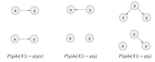
To compute p(y|do(x)), we need a causal diagram that encodes causal relationships between variables. The following picture show three causal diagrams and their corresponding p(y|do(x). Note that the arrow points from causes to effects.
要计算p(y | do(x)) ,我们需要一个因果图,该因果图编码变量之间的因果关系。 下图显示了三个因果图及其对应的p(y | do(x) 。请注意,箭头从原因指向结果。
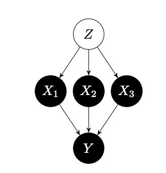
Examples to show the relationship between P(y|do(X)) and p(y|x) in three different causal diagrams, where z is the confounder [13] 在三个因果图中显示P(y | do(X))和p(y | x)之间关系的示例,其中z是混杂因素[13]In the paper [6], the authors argue that given a simple causal structure with a latent common cause Z as below, the observational conditional p(y|x1) does not correctly describe how Y changes after intervening on X1. The authors suggest using Interventional Conditional distribution p(y|do(x1) instead, which in this case is the marginal distribution.
在论文[6]中,作者认为,给定具有潜在共同原因Z的简单因果结构如下,观察条件p(y | x1)不能正确描述Y干预X1后的变化。 作者建议使用介入条件分布p(y | do(x1)代替,在这种情况下为边际分布。
Consider a causal structure where we have a common cause Z [Image Src: [6]] 考虑一个因果结构,其中我们有一个共同原因Z [Image Src:[6]]4.2。 边际与条件分布 (4.2. Marginal vs. Conditional distribution)
So, we have two distributions in hand that we can sample the absent features: Conditional Distribution (Eq. 9 in [1]) and Marginal Distribution (Eq. 11 in [1]). Marginal distribution can give us causality, but it has its own issue though. Let’s consider each option:
因此,我们手头有两个分布可以对不存在的特征进行采样:条件分布([1]中的方程9 )和边际分布([1]中的方程11 )。 边际分布可以使我们具有因果关系,但是它有其自身的问题。 让我们考虑每个选项:
Drawn from Marginal distribution: By doing this, we are making an assumption that the features are independent. The reason behind the assumption is that it can help us easier to calculate the approximation. Besides, the assumption also makes sense in terms of causal inference. In other words, in this case, SHAP can provide the causality [4, 15].
从边际分布得出:通过这样做,我们假设这些要素是独立的 。 该假设背后的原因是它可以帮助我们更轻松地计算近似值。 此外,该假设在因果推理方面也很有意义。 换句话说,在这种情况下,SHAP可以提供因果关系[4,15]。
However, in practice, the assumption on feature independence may not true in the data, and it can hurt the approximation [4]. When the assumption is wrong, we will end up creating unrealistic data points [7]. For example, to predict house prices, we have some features of the house as input data. Let’s say the first feature is
但是,实际上,关于特征独立性的假设可能在数据中并不正确,并且可能会损害近似值[4]。 当假设错误时,我们最终将创建不切实际的数据点[7]。 例如,为了预测房价,我们将房屋的某些功能作为输入数据。 假设第一个功能是
the area of the house, with 1000 square meters, and we sample values for num_of_rooms, an absent feature. If we sample num_of_rooms = 1 room for this data point, it would be unlikely and seems to be fake for such a big house like that.
占地 1000平方米的房屋面积,我们对num_of_rooms的值(不存在的特征)进行采样 。 如果我们为该数据点采样num_of_rooms = 1个房间,那么对于像这样的大房子来说是不可能的,而且似乎是假的。
- Drawn from Conditional distribution: It can solve the problem of correlated in marginal distribution, but it introduces a different problem in terms of causal inference. Conditional distribution violates the shape value properties because features which do not influence the prediction can still get different SHAP value rather than zero[7]. Thus, SHAP can not be a causality model if we use conditional distribution [4, 6]. 从条件分布中得出:它可以解决边际分布中的相关问题,但是在因果推理方面引入了另一个问题。 条件分布违反了形状值属性,因为不影响预测的特征仍然可以得到不同的SHAP值,而不是零[7]。 因此,如果我们使用条件分布[4,6],则SHAP不能成为因果模型。
What is the “right” distribution to use? Actually, there is a trade-off between True to the Model and True to the Data [9], and there may be no silver bullet here. In SHAP package, Marginal distributions are used as default when having the background data, and Conditional distributions can be used in Tree-based models when there’s no dataset available.
什么是使用的“正确”发行版? 实际上, 对模型的 正确与对数据的正确 [9]之间需要权衡取舍,这里可能没有灵丹妙药。 在SHAP程序包中,具有背景数据时将默认使用边际分布,而当没有可用数据集时,可以在基于树的模型中使用条件分布。
Consider the following piece of code of SHAP to explain a tree-based model. In the first line, we create a TreeExplainer object to explain a tree-based model. We put the model that needed to explain as the first parameter, and the data is the background dataset, usually X_train. In this case, SHAP can fill out absent features from the dataset (Marginal distribution). Otherwise, when the background data is not available, SHAP just follows the trees and use the number of training examples that went down each leaf to represent the background distribution (Conditional distribution) [12].
考虑下面的SHAP代码来解释基于树的模型。 在第一行中,我们创建一个TreeExplainer对象来解释基于树的模型。 我们将需要解释的模型作为第一个参数,数据是背景数据集,通常是X_train 。 在这种情况下,SHAP可以填充数据集中的缺失特征(边际分布)。 否则,当背景数据不可用时,SHAP会紧随树木,并使用沿着每片叶子下降的训练示例数来表示背景分布(条件分布)[12]。
explainer = shap.TreeExplainer(model = lgbm_model, data = X_train)shap_values = explainer.shap_values(X)
解释器= shap.TreeExplainer(模型= lgbm_model,数据= X_train)shap_values =解释器.shap_values(X)
5.功能在火车或测试仪上的重要性? (5. Feature importance on train or test set?)
At the code in the previous section, we use explainer.shap_values(X) (line 2). What should we put in X? Should it be X_train or X_test?
在上一节的代码中,我们使用了explorer.shap_values(X) (第2行)。 我们应该在X中输入什么? 应该是X_train还是X_test ?
It depends on the purpose of what to explain.
这取决于要解释的目的。
Let’s say we have a model which overfits on the train data. In other words, it’s useless when predicting new datasets.
假设我们有一个模型可以拟合火车数据。 换句话说,它在预测新数据集时没有用。
If we care about which features have the most influence on the model, just go with the train set for feature importance.
如果我们关心哪些特征对模型的影响最大,则只需训练一下特征就可以了。
Otherwise, if we expect the model is kind of garbage, it should have all zero(s) in terms of feature importance for all the features, the test set is the way to go.
否则,如果我们期望模型是一种垃圾,那么就所有特征的特征重要性而言,模型应全为零, 因此测试集是必经之路。
6.一些SHAP模型 (6. Some SHAP models)
For the full list of models available in SHAP, you can take a look at SHAP’s documents [12]. Here are some common models provided by the SHAP package.
有关SHAP中可用模型的完整列表,您可以查看SHAP的文档[12]。 这是SHAP软件包提供的一些常见模型。
6.1。 不可知模型 (6.1. Model-Agnostic)
Model-Agnostic explainers can explain any models. That being said, we need a function to map the input to the output.
与模型无关的解释器可以解释任何模型。 话虽这么说,我们需要一个函数将输入映射到输出。
KernelExplainer: based on LIME + a mathematical way to pick parameters. It uses marginal distribution to fill the absent features.
KernelExplainer:基于LIME +一种选择参数的数学方法。 它使用边际分布来填充缺失的特征。
6.2。 特定型号 (6.2. Model-Specific)
Model-Specific explainers can apply for a specific class of models. To explain the model, it needs to know how the model works.
特定于模型的解释器可以申请特定类别的模型。 为了解释模型,它需要知道模型是如何工作的。
TreeExplainer: Leveraging the internal structure of tree-based models (e.g., XGBoost, LightGBM, CatBoost) to speed up the running time. If we can provide the background dataset, it will use the dataset to sample the absent features. Otherwise, it represents the background distribution by looking at the number of training examples that went down each leaf [12].
TreeExplainer :利用基于树的模型(例如 XGBoost,LightGBM,CatBoost)的内部结构来加快运行时间。 如果我们可以提供背景数据集,它将使用数据集对缺少的特征进行采样。 否则,它通过查看每个叶子上的训练示例数量来表示背景分布[12]。
Deep Networks+ DeepSHAP: Based on DeepLIFT. DeepLIFT can approximate SHAP values in deep neural networks with some assumptions.
深度网络+ DeepSHAP :基于DeepLIFT 。 DeepLIFT可以通过一些假设在深度神经网络中近似SHAP值。
Deep Networks+ DeepSHAP: Based on DeepLIFT. DeepLIFT can approximate SHAP values in deep neural networks with some assumptions.+ GradientExplainer: Based on IntegratedGradient, and SmoothGradient
深度网络+ DeepSHAP :基于DeepLIFT 。 DeepLIFT可以通过一些假设在深度神经网络中近似SHAP值。 + GradientExplainer :基于IntegratedGradient和SmoothGradient
7. SHAP的优缺点 (7. Pros and Cons of SHAP)
7.1。 优点 (7.1. Advantages)
- SHAP has a solid theoretical foundation in game theory to come up with an explanation. SHAP在博弈论中具有扎实的理论基础,可以提出一个解释。
SHAP introduces a way to connect LIME and Shapley values so that we can have a good method (KernelExplainer) to explain any model.
SHAP引入了一种连接LIME和Shapley值的方法,因此我们可以有一个很好的方法( KernelExplainer)来解释任何模型。
- SHAP can explain to an individual level, we can also aggregate the results to get a global explanation. SHAP可以对个人进行解释,我们也可以汇总结果以获得全局解释。
SHAP has a fast implementation of tree-based models (TreeExplainer). The fast computation helps SHAP become popular and well used.
SHAP具有基于树的模型( TreeExplainer)的快速实现。 快速的计算有助于SHAP变得流行和被很好地使用。
7.2。 缺点 (7.2. Disadvantages)
The main weakness of SHAP in my opinion is the long-running time of KernelExplainer. It is quite slow when we’re dealing with a big dataset.
我认为SHAP的主要缺点是KernelExplainer的运行时间较长 。 当我们处理一个大数据集时,它相当慢。
8.结论 (8. Conclusion)
SHAP is a great tool for understanding any Machine Learning models. Among other tools, SHAP is my favorite. When I’m dealing with tree-based models, SHAP is the go-to method of mine.
SHAP是了解任何机器学习模型的好工具。 在其他工具中,SHAP是我的最爱。 当我处理基于树的模型时,SHAP是我的首选方法。
SHAP repository on Github is quite active as it’s updated frequently. I strongly recommend going to the notebook from SHAP’s author [15] to see the insights that SHAP can bring up with cool visualization techniques. For further reading, there are some other good tutorials that you can take a look [7, 10, 16, 17, 18, 19].
Github上的SHAP存储库非常活跃,因为它经常更新。 我强烈建议您去看SHAP的作者[15]的笔记本 ,看看SHAP可以通过出色的可视化技术带来的见解。 为了进一步阅读,还有其他一些不错的教程,您可以看一下[7,10,16,17,17,18,19]。
Image Src: [15]] Image Src:[15] ]参考资料 (REFERENCES)
[1] [SHAP main paper (2017)] A Unified Approach to Interpreting Model Predictions: http://papers.nips.cc/paper/7062-a-unified-approach-to-interpreting-model-predictions.pdf
[1] [SHAP主要论文(2017年)]解释模型预测的统一方法: http : //papers.nips.cc/paper/7062-a-unified-approach-to-interpreting-model-predictions.pd f
[2] [Tree SHAP paper (2018)] Consistent Individualized Feature Attribution for Tree Ensembles: https://arxiv.org/pdf/1802.03888.pdf
[2] [Tree SHAP论文(2018年)]对树木乐团的一致个性化特征归因: https ://arxiv.org/pdf/1802.03888.pdf
[3] [Improvement/Update on Tree SHAP paper — Nature MI (2020)] From local explanations to global understanding with explainable AI for trees: https://rb.gy/uzcuwj
[3] [关于“树木SHAP”文件的改进/更新-Nature MI(2020)]从本地解释到全球理解以及可解释的树木AI: https : //rb.gy/uzcuwj
[4] Discussion on conditional vs. marginal distribution: https://github.com/christophM/interpretable-ml-book/issues/142
[4]关于条件分布与边际分布的讨论: https : //github.com/christophM/interpretable-ml-book/issues/142
[5] Another discussion on conditional vs. marginal distribution: https://github.com/slundberg/shap/issues/882
[5]关于条件与边际分布的另一讨论: https : //github.com/slundberg/shap/issues/882
[6] Feature relevance quantification in explainable AI: A causality problem (2019): https://arxiv.org/pdf/1910.13413v1.pdf
[6]可解释的AI中的特征相关性量化:因果关系问题(2019): https : //arxiv.org/pdf/1910.13413v1.pdf
[7] [Book] Interpretable Machine Learning: https://christophm.github.io/interpretable-ml-book/shap.html
[7] [书籍]可解释的机器学习: https : //christophm.github.io/interpretable-ml-book/shap.html
[8] SHAP Package: https://github.com/slundberg/shap
[8] SHAP软件包: https : //github.com/slundberg/shap
[9] True to the Model or True to the Data? (2020) https://arxiv.org/pdf/2006.16234.pdf
[9]对模型适用还是对数据适用? (2020) https://arxiv.org/pdf/2006.16234.pdf
[10] [Kaggle’s course] Machine Learning Explainability https://www.kaggle.com/learn/machine-learning-explainability
[10] [Kaggle的课程]机器学习的可解释性https://www.kaggle.com/learn/machine-learning-explainability
[11] Shapley, Lloyd S. “A value for n-person games”: http://www.library.fa.ru/files/Roth2.pdf
[11] Shapley,Lloyd S.“ n人游戏的价值”: http : //www.library.fa.ru/files/Roth2.pdf
[12] SHAP documents: https://shap.readthedocs.io/en/stable/
[12] SHAP文件: https ://shap.readthedocs.io/en/stable/
[13] [Tutorial on Causal Inference] Illustrating Interventions via a Toy Example: https://www.inference.vc/causal-inference-2-illustrating-interventions-in-a-toy-example/
[13] [因果推理教程]通过玩具示例来说明干预: https : //www.inference.vc/causal-inference-2-illustrating-interventions-in-a-toy-example/
[14] [Lecture on Causal Inference] Ferenc Huszár Causal Inference in Everyday Machine Learning: https://youtu.be/HOgx_SBBzn0?list=PLzERW_Obpmv_nwp3WuATOY9mguv28Xd_R&t=1633
[14] [因果推理讲座]日常机器学习中的FerencHuszár因果推理: https ://youtu.be/HOgx_SBBzn0?list=PLzERW_Obpmv_nwp3WuATOY9mguv28Xd_R&t=1633
[15] SHAP tutorial from its author: https://github.com/slundberg/shap/blob/master/notebooks/general/Explainable AI with Shapley Values.ipynb
[15]作者的SHAP教程: https : //github.com/slundberg/shap/blob/master/notebooks/general/具有Shapley Values.ipynb的可解释AI
[16] [Good explanations and a great example on calculating SHAP for tree model] Interpreting complex models with SHAP values: https://medium.com/@gabrieltseng/interpreting-complex-models-with-shap-values-1c187db6ec83
[16] [有关为树模型计算SHAP的很好的解释和很好的示例]用SHAP值解释复杂的模型: https ://medium.com/@gabrieltseng/interpreting-complex-models-with-shap-values-1c187db6ec83
[17] [Tutorial on Tree SHAP from its author] Interpretable Machine Learning with XGBoost: https://towardsdatascience.com/interpretable-machine-learning-with-xgboost-9ec80d148d27
[17] [作者编写的Tree SHAP教程]使用XGBoost的可解释机器学习: https ://towardsdatascience.com/interpretable-machine-learning-with-xgboost-9ec80d148d27
[18] Interpretable Machine Learning with Python: http://savvastjortjoglou.com/intrepretable-machine-learning-nfl-combine.html
[18]使用Python的可解释机器学习: http : //savvastjortjoglou.com/intrepretable-machine-learning-nfl-combine.html
[19] Explain Your Model with the SHAP Values: https://towardsdatascience.com/explain-your-model-with-the-shap-values-bc36aac4de3d
[19]使用SHAP值解释模型: https ://towardsdatascience.com/explain-your-model-with-the-shap-values-bc36aac4de3d
翻译自: https://medium.com/ai-in-plain-english/understanding-shap-for-interpretable-machine-learning-35e8639d03db
可解释机器学习
