可变性卷积(Deformable Convolution network)系列论文学习
Deformable Convolution network
0.摘要
iccv2017
作者觉得传统的卷积感受野太小了,如果进行pooling减少图片的尺寸,在进行卷积肯定会损失很多信息,论文太偏理论,比较难阅读,但是代码写的不错。
可变性卷积和空洞卷积有点类似,从周围的像素点中提取信息。作者一共提供了两种新的方法:可变性卷积和可变性池化(原理都是一样的)
1.可变形网络
1.1可变形卷积
b中的图是学习后的产生的可变形卷积,而cd是人工设计的特殊的可变形卷积
普通卷积和可变性卷积区别(y是输出,p是位置信息,w权重,x输入):
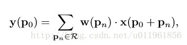
在普通卷积的基础上加上偏移量offsets :
![]()

由于在图片像素整合时,需要对像素进行偏移操作,偏移量的生成会产生浮点数类型,而偏移量又必须转换为整形,直接对偏移量取整的话无法进行反向传播,这时采用双线性差值的方式来得到对应的像素。所以最终的双线性插值:

![]()
反向传播的过程(一个很麻烦的偏微分):


偏移量是通过卷积学习到的,有一个额外的conv层来学习offset,共享input feature maps。然后input feature maps和offset共同作为deformable conv层的输入,deformable conv层操作采样点发生偏移,再进行卷积。
有一点像观众自注意力,带有一点注意力,作者把这中机制叫做自适应感受野:

普通卷积和可变形卷积在特征提取上的直观区别:

代码:
class ConvOffset2D(Conv2D):
    """ConvOffset2D

    Convolutional layer responsible for learning the 2D offsets and output the
    deformed feature map using bilinear interpolation

    Note that this layer does not perform convolution on the deformed feature
    map. See get_deform_cnn in cnn.py for usage
    """

    def __init__(self, filters, init_normal_stddev=0.01, **kwargs):
        """Init

        Parameters
        ----------
        filters : int
            Number of channel of the input feature map
        init_normal_stddev : float
            Normal kernel initialization
        **kwargs:
            Pass to superclass. See Con2D layer in Keras
        """

        self.filters = filters
        super(ConvOffset2D, self).__init__(
            self.filters * 2, (3, 3), padding='same', use_bias=False,
            kernel_initializer=RandomNormal(0, init_normal_stddev),
            **kwargs
        )

    def call(self, x):
        """Return the deformed featured map"""
        x_shape = x.get_shape()
        offsets = super(ConvOffset2D, self).call(x)

        # offsets: (b*c, h, w, 2)
        offsets = self._to_bc_h_w_2(offsets, x_shape)

        # x: (b*c, h, w)
        x = self._to_bc_h_w(x, x_shape)

        # X_offset: (b*c, h, w)
        x_offset = tf_batch_map_offsets(x, offsets)

        # x_offset: (b, h, w, c)
        x_offset = self._to_b_h_w_c(x_offset, x_shape)

        return x_offset

    def compute_output_shape(self, input_shape):
        """Output shape is the same as input shape

        Because this layer does only the deformation part
        """
        return input_shape

    @staticmethod
    def _to_bc_h_w_2(x, x_shape):
        """(b, h, w, 2c) -> (b*c, h, w, 2)"""
        x = tf.transpose(x, [0, 3, 1, 2])
        x = tf.reshape(x, (-1, int(x_shape[1]), int(x_shape[2]), 2))
        return x

    @staticmethod
    def _to_bc_h_w(x, x_shape):
        """(b, h, w, c) -> (b*c, h, w)"""
        x = tf.transpose(x, [0, 3, 1, 2])
        x = tf.reshape(x, (-1, int(x_shape[1]), int(x_shape[2])))
        return x

    @staticmethod
    def _to_b_h_w_c(x, x_shape):
        """(b*c, h, w) -> (b, h, w, c)"""
        x = tf.reshape(
            x, (-1, int(x_shape[3]), int(x_shape[1]), int(x_shape[2]))
        )
        x = tf.transpose(x, [0, 2, 3, 1])
        return x
1.2可变形池化
标准池化:
可变形池化:
1.3网络结构
作者在文章并没有写,只能通过代码来理解,只知道他是基于cnn,用mxnet框架写的
def get_deform_cnn(trainable):
    inputs = l = Input((28, 28, 1), name='input')

    # conv11
    l = Conv2D(32, (3, 3), padding='same', name='conv11', trainable=trainable)(l)
    l = Activation('relu', name='conv11_relu')(l)
    l = BatchNormalization(name='conv11_bn')(l)

    # conv12
    l_offset = ConvOffset2D(32, name='conv12_offset')(l)
    l = Conv2D(64, (3, 3), padding='same', strides=(2, 2), name='conv12', trainable=trainable)(l_offset)
    l = Activation('relu', name='conv12_relu')(l)
    l = BatchNormalization(name='conv12_bn')(l)

    # conv21
    l_offset = ConvOffset2D(64, name='conv21_offset')(l)
    l = Conv2D(128, (3, 3), padding='same', name='conv21', trainable=trainable)(l_offset)
    l = Activation('relu', name='conv21_relu')(l)
    l = BatchNormalization(name='conv21_bn')(l)

    # conv22
    l_offset = ConvOffset2D(128, name='conv22_offset')(l)
    l = Conv2D(128, (3, 3), padding='same', strides=(2, 2), name='conv22', trainable=trainable)(l_offset)
    l = Activation('relu', name='conv22_relu')(l)
    l = BatchNormalization(name='conv22_bn')(l)

    # out
    l = GlobalAvgPool2D(name='avg_pool')(l)
    l = Dense(10, name='fc1', trainable=trainable)(l)
    outputs = l = Activation('softmax', name='out')(l)

    return inputs, outputs


下面一节说在参数量上的优势
2.实验结果


可以看出在几乎不增加参数量与运行时间的情况下,论文的方法带来了较大的性能提升。可以使用分组卷积来减少模型的规模。