HW2: Numpy for Multi-Layer Neural Network

Before

        This homework is intended to give you an introduction to building, training, and testing neural network models. You will not only be exposed to using Python packages to build a neural network from scratch, but also the mathematical aspects of backpropagation and gradient descent. While in practical scenarios, you won’t necessarily have to implement neural networks from scratch (as you will see in future labs and assignments), this assignment aims at giving you a rudimentary idea of what goes on under the hood in packages such as TensorFlow and Keras. In this assignment, you will use the MNIST handwritten digits dataset to train a simple classification neural network using batch learning and evaluate your model.

中文（Chinese）： http://t.csdn.cn/2AyUX

---

Link to this article .pdf file 

---------------------------------------------------------------------------------------------------------------------------------

password：v6zc 

https://pan.baidu.com/s/1_qFbN0Nhc8MNYCHEyTbkLg%C2%A0

---

HW2: Numpy for Multi-Layer Neural Network

Before

Conceptual Questions

Getting the Stencil

Getting the Data

Assignment Overview

Before Starting

1. Preprocessing the Data

2. One Hot Encoding

3. Core Abstractions

4. Layers

5. Activation Functions

6. Filling in the model

7. Loss Function

8. Optimizers

9. Accuracy metrics

10. Train and Test

11. Visualizing Results

CS1470 Students

CS2470 Students

IMPORTANT!

---

Conceptual Questions

Please submit the Conceptuals Questions on Gradescope under hw2-mlp conceptual .

You must type your submissions and upload a PDF. We recommend using LaTeX.

Getting the Stencil

Github Classroom Link with Stencil Code!

Guide on GitHub and GitHub Classroom

Getting the Data

You can use download.sh for downloading the data. You can run a bash script with the

command ./script_name.sh (ex: bash ./download.sh ). This is similar to HW1. Setup

Work off of the stencil code provided, but do not change the stencil except where specified.

Doing so may cause incompatibility with the autograder. Don’t change any method signatures!

This assignment requires NumPy and Matplotlib. You should already have this from HW1. Also

check the virtual environment guide to set up TensorFlow 2.5 on your local machine. Feel free to

reference this guide if you have to work through colab.

Assignment Overview

In this assignment, you will be constructing a Keras mimic, Beras (haha funny name), and will

make a sequential model specification that mimics the Tensorflow/Keras API. The Python

notebook associated with this homework is meant for you to explore an example implementation

so that you can build on it yourself! There are no TODOs for you to work on in the notebook ;

rather, the testing is done by running the main method of assignment.py .

Our stencil provides a model class with several methods and hyperparameters you need to use

for your network. You will also answer conceptual questions related to the assignment and class

material (don’t forget to answer the 2470-only questions if you’re a 2470 student!). You should

include a brief README with your model's accuracy and any known bugs.

Before Starting

This homework assignment is due two weeks from release. Labs 1-3 provide great practice for

this assignment, so you can wait a little for them if you get stuck. Specifically:

-

Implementing Callable/Diffable Components : The skills you need in order to do this

can be found by working through Lab 1 . This includes comfort with mathematical

notation, matrix operations, and the logic behind call and gradient methods.

-

Implementing Optimizers: You can implement the BasicOptimizer class just by

following the logic from the gradient_descent method in lab 1. The other optimizers

(i.e. Adam, RMSProp) will be covered in Lab 2: Optimizers .

-

Using batch_step and GradientTape: You can figure out how to use these to train your

model based on the assignment instructions and your implementations of these. With

that said, they do mimic the Keras API. You’ll learn about all this in Lab 3: Intro to

Tensorflow . If your lab is after the due date, it should be fine; just skim over the

complementary notebook associated with the lab.

Feel free to start off by doing what you can and then add onto it as you learn more about deep

learning and realize that the same concepts you learn in the class can actually be used here!

Do not get discouraged, and try to have fun! Roadmap

For this assignment, we'll walk you through the pipeline of training a neural net, including the

structure of the model class and the methods you will have to fill in.

1. Preprocessing the Data

Note: Code for preprocessing should be pulled in from HW1.

Before training a network, you will need to clean your data. This includes retrieving,

altering, and formatting the data into the inputs for your network. For this assignment,

you will be working on the MNIST dataset. It can be downloaded through the

download.sh script, but it’s also linked here (ignore that it says hw1; we’re using this

dataset for hw2 this time!). The original data source is here .

You should train your network using only the training data and then test your network's

accuracy on the testing data. Your program should print its accuracy over the test

dataset upon completion.

2. One Hot Encoding

Before training or testing your model, you will need to “one-hot” encode your class labels

so that the model can optimize towards predicting any desired class. Note that the class

labels by themselves are simply categories and do not mean anything numerically. In the

absence of one-hot encoding, your model might learn some natural ordering between

the different class labels based on the labels (which are arbitrary).

For example, let’s say there’s a data point A which corresponds to label ‘2’ and a data

point B which corresponds to label ‘7’. We don’t want the model to somehow learn that B

has a higher weightage than A simply because, numerically speaking, 7 > 2.

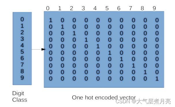
To one-hot encode your class labels, you will

have to convert your 1-dimensional label vector

into a vector of size num_classes (where

num_classes is the total number of classes in

your dataset). For the MNIST dataset, it looks

something like the matrix on the right:

You have to fill out the following method in Beras/onehot.py

● fit() : [TODO] In this function you need to fetch all the unique labels in the

data (store this in self.uniq ) and create a dictionary with labels as the keys

and their corresponding one hot encodings as values. Hint: You might want to

look at np.eye() to get the one-hot encodings. Ultimately, you will store this

dictionary in self.uniq2oh .

● forward() : In this function, we pass a vector of all the actual labels in the

training set and call fit() to populate the uniq2oh dictionary with unique

labels and their corresponding one-hot encoding and then use it to return an

array of one-hot encoded labels for each label in the training set. This function

has already been filled out for you!

● inverse() : In the function, we reverse the one-hot encoding back to the actual

label. This has already been done for you.

For example, if we have labels X and Y with one-hot encodings of [1,0] and [0,1], we’d

want to create a dictionary as follows: {X: [1,0], Y: [0,1]}. As shown in the image above,

for MNIST, you will have 10 labels, so your dictionary should have ten entries!

You may notice that some classes inherit from Callable or Diffable. More on this

in the next section!

3. Core Abstractions

Consider the following abstract classes of modules. Be sure to play around with the

Python notebook associated with this homework to get a good grip of the core

abstraction modules defined for you in Beras/core.py ! The notebook is exploratory in

nature (it is NOT required and all of the code is given) and will provide you with lots of

insights into understanding and using these class abstractions! Note that these modules

are very similar to the Tensorflow/Keras API.

Callable: A function with a well-defined forward function. These are the ones you’ll need

to implement:

        ● CategoricalAccuracy (./metrics.py): Computes the accuracy of predicted

probabilities against a list of ground-truth labels. As accuracy is not optimized for,

there is no need to compute its gradient. Furthermore, categorical accuracy is

piecewise discontinuous, so the gradient would technically be 0 or undefined.

        ● OneHotEncoder (./onehot.py) : You can one-hot encode a class instance into a

probability distribution to optimize for classifying into discrete options

Diffable: A callable which can also be differentiated. We can use these in our pipeline

and optimize through them! Thus, most of these classes are made for use in your neural

network layers. These are the ones you’ll need to implement: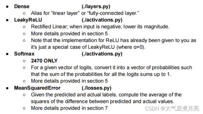

Example: Consider a Dense layer instance. Let s represents the input size (source), d

represents the output size (destination), and b represents the batch size. Then:

GradientTape: This class will function exactly like tf.GradientTape() (See lab 3).

You can think of a GradientTape as a logger. Every time an operation is performed within

the scope of a GradientTape, it records which operation occurred. Then, during

backprop, we can compute the gradient for all of the operations. This allows us to

differentiate our final output with respect to any intermediate step. When operations are

computed outside the scope of GradientTape, they aren’t recorded, so your code will

have no record of them and cannot compute the gradients.

You can check out how this is implemented in core! Of course, Tensorflow’s gradient

tape implementation is a lot more complicated and involves constructing a graph.

 ● [TODO] Implement the gradient method, which returns a list of gradients corresponding to the list of trainable weights in the network. Details in the code.

4. Layers

For the purposes of this assignment, you will implement the Dense layer to use in your

sequential model in Beras/layers.py . You have to fill in the following methods.

● forward() : [TODO] Implement the forward pass and return the outputs.

● weight_gradients() : [TODO] Calculate the gradients with respect to the

weights and the biases. This will be used to optimize the layer .

● input_gradients() : [TODO] Calculate the gradients with respect to the

layer inputs. This will be used to propagate the gradient to previous layers.

● _initialize_weight() : [TODO] Initialize the dense layer’s weight values.

By default, initialize all the weights to zero (usually a bad idea, by the way). You

are also required to allow for more sophisticated options (when the initializer is

set to normal, xavier, and kaiming). Follow Keras math assumptions!

        ○ Normal: Pretty self-explanatory, a unit normal distribution.

        ○ Xavier Normal: Based on keras.GlorotNormal .

        ○ Kaiming He Normal: Based on Keras.HeNormal .

You may find np.random.normal helpful while implementing these. The TODOs

provide some justification for why these different initialization methods are necessary but

for more detail, check out this website ! Feel free to add more initializer options!

5. Activation Functions

In this assignment, you will be implementing two major activation functions, namely,

LeakyReLU and Softmax in Beras/activations.py . Since ReLU is a special case

of LeakyReLU , we have already provided you with the code for it.

● LeakyReLU()

        ○ forward() : [TODO] Given input x , compute & return LeakyReLU(x) .

        ○ input_gradients() : [TODO] Compute & return the partial with

        respect to inputs by differentiating LeakyReLU .

● Softmax() : (2470 ONLY)

        forward(): [TODO] Given input x , compute & return Softmax(x) .

        Make sure you use stable softmax where you subtract max of all entries

        to prevent overflow/undvim erflow issues.

        ○ input_gradients() : [TODO] Partial w.r.t. inputs of Softmax() .

6. Filling in the model

With these abstractions in mind, let’s create a pipeline for our sequential deep learning

model. You can find the SequentialModel class in assignment.py where you will

initialize your neural network’s layers, parameters (weights and biases), and

hyperparameters (optimizer, loss function, learning rate, accuracy function, etc.). The

SequentialModel class inherits from Beras/model.py , where you’ll find many

useful methods. This will also contain functions that fit the model to your data and

evaluate the performance of your model:

● compile() : Initialize the model optimizer, loss function, & accuracy function,

which are fed in as arguments, for your SequentialModel instance to use.

● fit() : Trains your model to associate input to outputs. Training is repeated for

each epoch, and the data is batched based on argument. It also computes

batch_metrics , epoch_metrics , and the aggregated agg_metrics that

can be used to track the training progress of your model.

● evaluate() : [TODO] Evaluate the performance of the final model using the

metrics mentioned above during the testing phase. It’s almost identical to the

fit() function; think about what would change between training and testing).

● call() : [TODO] Hint: what does it mean to call a sequential model? Remember

that a sequential model is a stack of layers where each layer has exactly one

input vector and one output vector. You can find this function within the

SequentialModel class in assignment.py .

● batch_step() : [TODO] You will observe that fit() calls this function for each

batch. You will first compute your model predictions for the input batch. In the

training phase, you will need to compute gradients and update your weights

according to the optimizer you are using. For backpropagation during training,

you will use GradientTape from the core abstractions ( core.py ) to record

operations and intermediate values. You will then use the model's optimizer to

apply the gradients to your model's trainable variables. Finally, compute and

return the loss and accuracy for the batch. You can find this function within the

SequentialModel class in assignment.py .

We encourage you to check out keras.SequentialModel in the intro notebook

(under Exploring a possible modular implementation: TensorFlow/Keras ) and refer

to Lab 3 to get a feel for how we can work with gradient tapes in deep learning.

7. Loss Function

This is one of the most crucial aspects of model training. In this assignment, we will

implement the MSE or mean-squared error loss function. You can find your loss function

in Beras/losses.py .

● forward() : [TODO] Write a function that computes and returns the mean

squared error given the predicted and actual labels.

Hint: What is MSE?

Given the predicted and actual labels, MSE is the average of the squares of the

differences between predicted and actual values.

● input_gradients() : [TODO] Compute and return the gradients. Use

differentiation to derive the formula for these gradients.

8. Optimizers

In the Beras/optimizers.py file make sure to implement the optimization for each of

the different types of optimizers. Lab 2 should help with this, so good luck!

● BasicOptimizer : [TODO] A simple optimizer strategy as seen in Lab 1.

● RMSProp : [TODO] Root mean squared error propagation.

● Adam : [TODO] A common adaptive motion estimation-based optimizer.

9. Accuracy metrics

Finally, to evaluate the performance of your model, you need to use appropriate

accuracy metrics. In this assignment, you will implement categorical accuracy in

Beras/metrics.py :

● forward() : [TODO] Return the categorical accuracy of your model given the

predicted probabilities and true labels. You should be returning the proportion of

predicted labels equal to the true labels, where the predicted label for an image is

the label corresponding to the highest probability. Refer to the internet or lecture

slides for categorical accuracy math!

10. Train and Test

Finally, using all the above primitives, you are required to build two models in

assignment.py:

● A simple model in get_simple_model() with at most one Diffable layer (e.g.,

Dense - ./layers.py ) and one activation function (look for them in

./activation.py ). This one is provided for you by default, though you can

change it if you’d like. The autograder will evaluate the original one though!

● A slightly more complex model in get_advanced_model() with two or more

Diffable layers and two or more activation functions. We recommend using Adam

optimizer for this model with a decently low learning rate.

For any hyperparameters you use (layer sizes, learning rate, epoch size, batch size,

etc.), please hardcode these values in the get_simple_model() and

get_advanced_model() functions. Do NOT store them under the main handler.

Once everything is implemented, you can use python3 assignment.py to run your

model and see the loss/accuracy!

11. Visualizing Results

We provided the visualize_metrics method for you to visualize how your loss and

accuracy changes after each batch using matplotlib. DO NOT EDIT THIS FUNCTION.

You should call this function in your main method after you store the loss and accuracy

per batch in an array, which would be passed into this function. This should plot line

graphs where the horizontal axis is the i'th batch and the vertical axis is the

loss/accuracy value of the batch. Calling this is OPTIONAL!

We've also provided the visualize_images method for you to visualize your

predictions against the true labels with matplotlib. This method is currently written with

the labels having a shape of [number of images, 1]. DO NOT EDIT THIS FUNCTION .

You should call this function with all your inputs and labels after training your model. The

function will randomly pick 500 samples from your input and will plot 10 correct and 10

incorrect classifications to help you visually interpret your model’s predictions! You

should do this last, after you have met the benchmark for test accuracy.

CS1470 Students

- Complete and Submit HW2 Conceptual

- Implement Beras per specifications and make a SequentialModel in assignment.py

- Test the model inside of main

- Get test accuracy >=85% on MNIST with default get_simple_model_components .

- Complete the Exploration notebook and export it to a PDF.

- The “HW2 Intro to Beras” notebook is just for your reference.

CS2470 Students

- Same as 1470 except:

- Implement Softmax activation function (forward pass and input_gradients )

- Get testing accuracy >95% on MNIST model from get_advanced_model_components .

- You will need to specify a multi-layered model, will have to explore

hyperparameter options, and may want to add additional features.

- Additional features may include regularization, other weight initialization

schemes, aggregation layers, dropout, rate scheduling, or skip connections. If

you have other ideas, feel free to ask publicly on Ed and we’ll let you know if they

are also ok.

- When implementing these features, try to mimic the Keras API as much as

possible. This will help significantly with your Exploration notebook.

- Finish 2470 components for Exploration notebook and conceptual questions.

Grading and Autograder Compatibility

Conceptual : You will be primarily graded on correctness, thoughtfulness, and clarity.

Code: You will be primarily graded on functionality. Your model should have an accuracy that is

at least greater than the threshold on the testing data. For 1470, this can be achieved with the

simple model parameterization provided. For 2470, you may need to experiment with

hyperparameters or develop some custom components.

Although you will not be graded on code style, you should not have an excessive number of

print statements in your final submission.

IMPORTANT! Please use vectorized operations when possible and limit the number of for loops

you use. While there is no strict time limit for running this assignment, it should typically be less

than 3 minutes. The autograder will automatically time out after 10 minutes. You will not receive

any credit for methods that use Tensorflow or Keras functions within them.

Notebook: The exploration notebook will be graded manually and should be submitted as a pdf

file. Feel free to use the “Notebooks to Latex PDFs.ipynb” notebook! Handing In

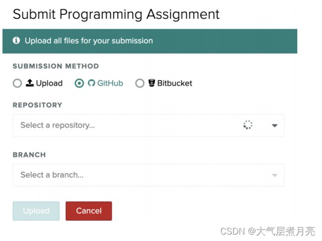
You should submit the assignment via Gradescope under the corresponding project assignment

by zipping up your hw2 folder (the path on Gradescope MUST be hw2/code/filename.py) or

through GitHub ( recommended ). To submit through GitHub, commit and push all changes to

your repository to GitHub. You can do this by running the following three commands ( this is a

good resource for learning more about them):

1. git add file1 file2 file3 (or -A)
2. git commit -m “commit message”
3. git push

After committing and pushing your changes to your repo (which you can check online if you're unsure if it worked), you can now just upload the repo to Gradescope! If you’re testing out code on multiple branches, you have the option to pick whichever one you want.

IMPORTANT!

1. Please make sure all your files are in hw2/code . Otherwise, the autograder will fail!

2. Delete the data folder before zipping up your code.

3. 2470 STUDENTS : Add a blank file named 2470student in the hw2/code directory!

The file should have no extension, and is used as a flag to grade 2470-specific requirements. If

you don’t do this, YOU WILL LOSE POINTS!

Thanks!