机器学习1.线性回归
从本部分开始,从头研究机器学习内容,并尽可能详细的介绍各种机器学习算法,尽可能做到完善,详细,明确。
线性回归算法
1.介绍
以一元一次函数为研究对象,形如y=wx+b,若给出(x,y)的一系列值,期望得到参数w,b的值,这里使用得工具为python及相关库,如numpy,pandas等。
2.引入封装好的库
import numpy as np
import matplotlib.pyplot as plt
3.生成数据
data = []  # 保存样本集的列表
for i in range(100):    # 循环采样100个点
    x = np.random.uniform(-10., 10.)    # 随机采样输入x
    eps = np.random.normal(0., 0.1)     # 采样高斯噪声
    y = 1.477 * x + 0.089 + eps         # 得到模型输出
    data.append([x, y])                 # 保存样本点
data = np.array(data)                   # 转换为2D numpy数组
# print(len(data))                      # 输出为100
# print(data[:,0],data[:,1])            # 其中x=data[:,0],y=data[:1]
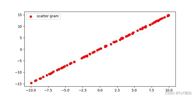
4.散点图可视化
# 散点图
# 绘图
# 1. 确定画布
plt.figure(figsize=(8, 4))  # figsize:确定画布大小

# 2. 绘图
plt.scatter(data[:,0],  # 横坐标
            data[:,1],  # 纵坐标
            c='red',  # 点的颜色
            label='scatter gram')  # 标签 即为点代表的意思
# 3.展示图形
plt.legend()  # 显示图例(标签)

plt.show()  # 显示所绘图形
5.定义MSE、梯度下降等
def mse(b, w, points):
    # 根据当前w,b参数计算方差损失
    totalError = 0
    for i in range(0, len(points)): # 循环迭代所有点
        x = points[i, 0]            # 获取i号点的输出x
        y = points[i, 1]            # 获取i号点的输出y
        totalError += (y - (w * x + b)) ** 2    # 计算差的平方,并累加
    return totalError/float(len(points))    # 将累加的误差求平均,得到均方差


def step_gradient(b_current, w_current, points, lr):  # 计算误差函数在所有点上的导数,并更新 w,b
    b_gradient = 0
    w_gradient = 0
    M = float(len(points))  # 总样本数
    for i in range(0, len(points)):
        x = points[i, 0]
        y = points[i, 1]
    # 误差函数对 b 的导数: grad_b = 2(wx+b-y)
        b_gradient += (2/M) * ((w_current * x + b_current) - y)
    # 误差函数对 w 的导数: grad_w = 2(wx+b-y)*x
        w_gradient += (2/M) * x * ((w_current * x + b_current) - y)
    # 根据梯度下降算法更新 w',b',其中 lr 为学习率
    new_b = b_current - (lr * b_gradient)
    new_w = w_current - (lr * w_gradient)
    return [new_b, new_w]


def gradient_descent(points, starting_b, starting_w, lr, num_iterations):
    # 循环更新 w,b 多次
    b = starting_b  # b 的初始值
    w = starting_w  # w 的初始值
    # 根据梯度下降算法更新多次
    #梯度下降法介绍:https://zhuanlan.zhihu.com/p/335191534
    for step in range(num_iterations):
        #  计算梯度并更新一次
        b, w = step_gradient(b, w, np.array(points), lr)
        loss = mse(b, w, points)  # 计算当前的均方差,用于监控训练进度
        if step % 50 == 0:  # 打印误差和实时的 w,b 值
            print(f"iteration:{step}, loss:{loss}, w:{w}, b:{b}")
    return [b, w]  # 返回最后一次的 w,b
6.完整代码
import numpy as np
import matplotlib.pyplot as plt
data = [] # 保存样本集的列表
for i in range(100): # 循环采样100个点
x = np.random.uniform(-10., 10.) # 随机采样输入x
eps = np.random.normal(0., 0.1) # 采样高斯噪声
y = 1.477 * x + 0.089 + eps # 得到模型输出
data.append([x, y]) # 保存样本点
data = np.array(data) # 转换为2D numpy数组
#print(data[:,0])
# 散点图
# 绘图
# 1. 确定画布
plt.figure(figsize=(8, 4)) # figsize:确定画布大小
# 2. 绘图
plt.scatter(data[:,0], # 横坐标
data[:,1], # 纵坐标
c='red', # 点的颜色
label='scatter gram') # 标签 即为点代表的意思
# 3.展示图形
plt.legend() # 显示图例(标签)
#plt.show() # 显示所绘图形
def mse(b, w, points):
# 根据当前w,b参数计算方差损失
totalError = 0
for i in range(0, len(points)): # 循环迭代所有点
x = points[i, 0] # 获取i号点的输出x
y = points[i, 1] # 获取i号点的输出y
totalError += (y - (w * x + b)) ** 2 # 计算差的平方,并累加
return totalError/float(len(points)) # 将累加的误差求平均,得到均方差
def step_gradient(b_current, w_current, points, lr): # 计算误差函数在所有点上的导数,并更新 w,b
b_gradient = 0
w_gradient = 0
M = float(len(points)) # 总样本数
for i in range(0, len(points)):
x = points[i, 0]
y = points[i, 1]
# 误差函数对 b 的导数: grad_b = 2(wx+b-y)
b_gradient += (2/M) * ((w_current * x + b_current) - y)
# 误差函数对 w 的导数: grad_w = 2(wx+b-y)*x
w_gradient += (2/M) * x * ((w_current * x + b_current) - y)
# 根据梯度下降算法更新 w',b',其中 lr 为学习率
new_b = b_current - (lr * b_gradient)
new_w = w_current - (lr * w_gradient)
return [new_b, new_w]
def gradient_descent(points, starting_b, starting_w, lr, num_iterations):
# 循环更新 w,b 多次
b = starting_b # b 的初始值
w = starting_w # w 的初始值
# 根据梯度下降算法更新多次
for step in range(num_iterations):
# 计算梯度并更新一次
b, w = step_gradient(b, w, np.array(points), lr)
loss = mse(b, w, points) # 计算当前的均方差,用于监控训练进度
if step % 50 == 0: # 打印误差和实时的 w,b 值
print(f"iteration:{step}, loss:{loss}, w:{w}, b:{b}")
return [b, w] # 返回最后一次的 w,b
def main():
# 加载训练集数据,这些数据是通过真实模型添加观测误差采样得到的
lr = 0.01 # 学习率
initial_b = 0 # 初始化 b 为 0
initial_w = 0 # 初始化 w 为 0
num_iterations = 1000
# 训练优化 1000 次,返回最优 w*,b*和训练 Loss 的下降过程
[b, w] = gradient_descent(data, initial_b, initial_w, lr, num_iterations)
loss = mse(b, w, data) # 计算最优数值解 w,b 上的均方差
print(f'Final loss:{loss}, w:{w}, b:{b}')
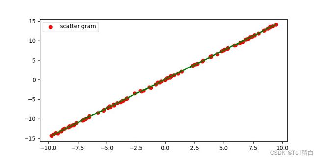
plt.plot(data[:,0], w*data[:,0]+b, color='g') #绘制拟合的函数图
plt.show()
main()
梯度下降、线性回归相关知识及公式推导如下链接:
公式推导
7.使用scikit-learn库
7.1 一元一次线性回归方程
# 1.引入相关库
import numpy as np
from sklearn.linear_model import LinearRegression
# 2.导入数据
x = np.array([5, 15, 25, 35, 45, 55]).reshape(-1,1) #x是二维的而y是一维的,因为在复杂一点的模型中,系数不只一个。
y = np.array([5, 20, 14, 32, 22, 38])
# 3.建立模型
model = LinearRegression().fit(x, y)  # 使用fit()训练参数
# 4.查看结果
r_sq = model.score(x, y)  #score()函数可以获得模型R的平方
print('coefficient of determination:', r_sq)  # 获得R的平方
print('intercept:', model.intercept_)  #方程常数项
print('slope:', model.coef_)  #方程系数
# 5.预测
x_new = np.arange(5).reshape(-1,1)
y_pred = model.predict(x_new)  #predict调用预测函数
print('predicted response:', y_pred, sep='\t')

#输出结果:
coefficient of determination: 0.715875613747954
intercept: 5.633333333333329
slope: [0.54]
predicted response:	[5.63333333 6.17333333 6.71333333 7.25333333 7.79333333]
7.2 二元一次线性回归方程
# 1.引入相关库
import numpy as np
from sklearn.linear_model import LinearRegression
# 2.导入数据
x = [[0, 1], [5, 1], [15, 2], [25, 5], [35, 11], [45, 15], [55, 34], [60, 35]]
y = [4, 5, 20, 14, 32, 22, 38, 43]
# 3.建立模型
model = LinearRegression().fit(x, y)  # 使用fit()训练参数
# 4.查看结果
r_sq = model.score(x, y)  #score()函数可以获得模型R的平方
print('coefficient of determination:', r_sq)  # 获得R的平方
print('intercept:', model.intercept_)  #方程常数项
print('slope:', model.coef_)  #方程系数
# 5.预测
x_new = np.arange(10).reshape((-1, 2))
y_pred = model.predict(x_new)  #predict调用预测函数
print('predicted response:', y_pred, sep='\t')

#输出结果:
coefficient of determination: 0.8615939258756775
intercept: 5.52257927519819
slope: [0.44706965 0.25502548]
predicted response:	[ 5.77760476  7.18179502  8.58598528  9.99017554 11.3943658 ]