This story is a walk-through of a notebook I uploaded on Kaggle. Originally, it only used machine learning models and since then I have added a couple of basic neural network models. The churn prediction topic has been extensively covered by many blogs on Medium and notebooks on Kaggle, however, there are very few using neural networks. The application of neural networks to structured data in itself is seldom covered in the literature. I learned neural networks through the deeplearning.ai specialization on Coursera and the documentation of Tensorflow with Keras.
这个故事是我在Kaggle上上传的笔记本的逐步介绍。 最初,它仅使用机器学习模型,从那时起,我添加了几个基本的神经网络模型。 流失预测主题已被Medium上的许多博客和Kaggle上的笔记本广泛涵盖,但是,很少使用神经网络。 在文献中很少涉及将神经网络本身应用于结构化数据。 我通过Coursera的deeplearning.ai专业知识以及Keras的Tensorflow文档学习了神经网络。
介绍 (Introduction)
Customer attrition or customer churn occurs when customers or subscribers stop doing business with a company or service. Customer churn is a critical metric because it is much more cost effective to retain existing customers than it is to acquire new customers as it saves cost of sales and marketing. Customer retention is more cost-effective as you’ve already earned the trust and loyalty of existing customers.
当客户或订户停止与公司或服务开展业务时,就会发生客户流失或客户流失。 客户流失率是一项关键指标,因为保留现有客户比获取新客户更具成本效益,因为它可以节省销售和营销成本。 客户保留率更具成本效益,因为您已经赢得了现有客户的信任和忠诚度。
There are various ways to calculate this metric as churn rate may represent the total number of customers lost, the percentage of customers lost compared to the company’s total customer count, the value of recurring business lost, or the percent of recurring value lost. However, in this dataset, it is defined as a binary variable for each customer and calculating the rate is not the objective. Thus the objective here is to identify and quantify the factors which influence churn rate.
有多种方法可以计算此指标,因为流失率可以代表丢失的客户总数,丢失的客户占公司总客户数的百分比,经常性业务损失的价值或经常性价值损失的百分比。 但是,在此数据集中,它被定义为每个客户的二进制变量,并且计算费率不是目标。 因此,这里的目的是识别和量化影响客户流失率的因素。
This is a fairly easy and beginner level project with fewer variables. It is not a useful application for neural networks as number of training examples are comparatively less but it is easy to understand neural networks using this.
这是一个相当简单的入门级项目,变量较少。 这对神经网络不是有用的应用程序,因为训练示例的数量相对较少,但是使用它可以很容易地理解神经网络。
探索性数据分析 (Exploratory Data Analysis)
The data cleaning steps are skipped here. Missing values were only minute and found in Total Charges column and thus dropped. No features were dropped owing to multi-collinearity as only few features are present.
此处跳过数据清理步骤。 缺少的值只有分钟,可以在“总费用”列中找到,因此被丢弃。 由于存在多个共线性,因此没有因多共线性而丢失任何特征。

The first step in data analysis is familiarizing yourself with the data variables, features and the target. This dataset contains 20 features and one target variable. The customer ID feature is a string identification, thus not useful for prediction.
数据分析的第一步是使自己熟悉数据变量,功能和目标。 该数据集包含20个要素和一个目标变量。 客户ID功能是字符串标识,因此对预测没有用。
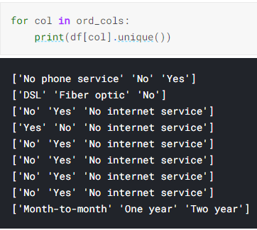
In the categorical features, some features are binary and some have exactly 3 unique values. On examining, it is noted that only Contract and Internet service have a different number of unique values in the categorical features. The ‘No internet service’ class could be assigned to ‘No’ as in some notebooks on Kaggle. However, dummy variables seem better encoding option instead as in former case there will be loss of data that the customer has chosen not to opt for a service despite having internet service. In case the number of features were larger, label encoding or mapping would be considered as then the one hot encoding would become a large sparse matrix.
在分类特征中,某些特征是二进制的,而某些特征恰好具有3个唯一值。 在检查时,请注意,只有合同和Internet服务在分类功能中具有不同数量的唯一值。 像在Kaggle上的某些笔记本中一样,可以将“没有互联网服务”类别分配为“否”。 但是,伪变量似乎是更好的编码选项,因为在前一种情况下,尽管有互联网服务,但客户选择不选择服务的数据将会丢失。 在特征数量较大的情况下,标签编码或映射将被认为是一种热编码将成为大型稀疏矩阵。
It is important to check the distribution of these features provided in our data to check for biases if the feature values are impartially distributed. A function such as below is used to plot the distributions.
重要的是要检查我们数据中提供的这些特征的分布,以检查特征值是否公平分布是否存在偏差。 下面的函数用于绘制分布。
def srt_dist(df=df,cols=cat_feats):
    fig, axes = plt.subplots(8, 2,squeeze=True)
    axes = axes.flatten()
    for i, j in zip(cols, axes):
        (df[i].value_counts()*100.0 /len(df)).plot.pie(autopct='%.1f%%',figsize =(10,37), fontsize =15,ax=j )
        j.yaxis.label.set_size(15)
srt_dist()

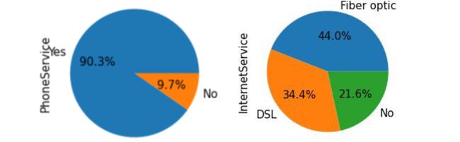
It is observed that very few are senior citizens, only 30% have dependents, and only 10% have no phone service. Thus, the correlations drawn from these variables can be doubted.
据观察,很少有老年人,只有30%有受抚养人,只有10%没有电话服务。 因此,可以怀疑从这些变量得出的相关性。
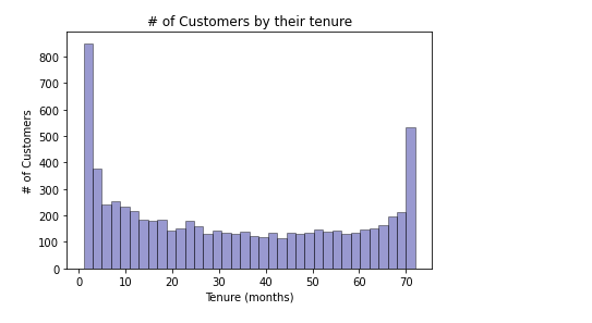

Naturally, month to month contract customers tenure lower than customer with two year contracts.
自然,月度合同客户的任期比具有两年期合同的客户的任期低。

Thus, the target variable has 73 % instances of ‘no-churn’. The machine learning models will be skewed because of this and will not perform as good on unseen data with more instances of ‘churn’.
因此,目标变量具有73%的“无搅动”实例。 因此,机器学习模型将出现偏差,并且在带有更多“搅动”实例的看不见的数据上表现不佳。
One method to counteract this imbalance of classes is using stratified cross validation, which makes folds with uniform proportions of the instances.
解决类的这种不平衡的一种方法是使用分层交叉验证,该交叉验证以均匀比例的实例进行折叠。
sns.pairplot(df,vars = ['tenure','MonthlyCharges','TotalCharges'], hue="Churn")
From the top row middle plot, it is observed that customers having lower tenure and higher monthly charges are tend to churn, with almost a linear relationship. It can be noted that as shown in the total charges distribution, the neural network model also indicates that customers with lower total charges churn. However this might be due to customers with higher tenure having more total charges over time.
从顶部的中间图可以看出,具有较低任期和较高月租费的客户趋于流失,几乎具有线性关系。 可以注意到,如总费用分布所示,神经网络模型还表明总费用较低的客户流失。 但是,这可能是由于使用期较长的客户随时间推移收取的总费用更高。
Also as you can see below; having month-to-month contract and fiber obtic internet have a really huge effect on churn probability.
就像你在下面看到的一样; 拥有月度合同和光纤互联网对客户流失率的影响非常大。
cat_feats=['gender', 'SeniorCitizen', 'Partner', 'Dependents','PhoneService','MultipleLines', 'InternetService', 'OnlineSecurity', 'OnlineBackup','DeviceProtection', 'TechSupport', 'StreamingTV', 'StreamingMovies','Contract', 'PaperlessBilling', 'PaymentMethod'] # As formed in notebook in upper blocks
fig,axes = plt.subplots(16)
axes = axes.flatten()
for i, j in zip(cat_feats, axes):
sortd = df.groupby([i])['Churn'].median().sort_values(ascending=False)
    j=sns.catplot(x=i,
                y='Churn',
                data=df,
                kind='bar')
    j.set_ylabels("Churn Probability")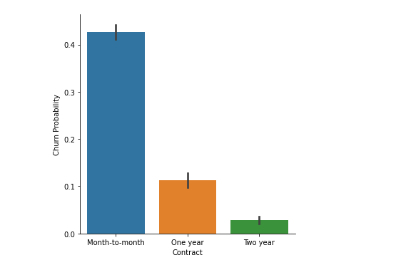
It is observed probability of churn is high for highly correlated features such as No partner or dependent, no tech support, month to month contract, etc.
对于高度相关的功能,例如没有合作伙伴或从属,没有技术支持,每月合同等,观察到客户流失的可能性很高。
造型 (Modelling)
The dataset is scaled according to MinMax scaler with range of 0 to 1 and the training set is the first 3993 observations according to the assignment.
根据MinMax缩放器对数据集进行缩放,范围为0到1,训练集是根据分配的前3993个观测值。
The below function was used for stratified cross validation.
以下功能用于分层交叉验证。
def stratified_cv(X, y, clf_class, shuffle=True,  **kwargs):
    stratified_k_fold = StratifiedKFold().split(X,y)
    y_pred = y.copy()
    for ii, jj in stratified_k_fold:
        Xtrain, Xtest = X.iloc[ii], X.iloc[jj]
        ytrain = y.iloc[ii]
        clf = clf_class(**kwargs)
        clf.fit(X_train,y_train)
        y_pred.iloc[jj] = clf.predict(Xtest)
    return y_predprint('Gradient Boosting Classifier:\n {}\n'.format(
    metrics.classification_report(y, stratified_cv(X, y,                                                  ensemble.GradientBoostingClassifier))))
print('Support vector machine(SVM):\n {}\n'.format(
    metrics.classification_report(y, stratified_cv(X, y, svm.SVC))))
print('Random Forest Classifier:\n {}\n'.format(
       metrics.classification_report(y, stratified_cv(X, y,                                                  ensemble.RandomForestClassifier))))
print('K Nearest Neighbor Classifier:\n {}\n'.format(
       metrics.classification_report(y, stratified_cv(X, y,                                                  neighbors.KNeighborsClassifier,n_neighbors=11))))
print('Logistic Regression:\n {}\n'.format(
       metrics.classification_report(y, stratified_cv(X, y,                                            linear_model.LogisticRegression))))
print('XGBoost Classifier:\n {}\n'.format(
     metrics.classification_report(y, stratified_cv(X, y,        XGBClassifier))))Code used for classification reports of ML model
Hyper parameter tuning of ML models
ML模型的超参数调整
For Random Forest, the number of estimators and max features per tree is tuned:
对于随机森林,调整每棵树的估计量和最大特征的数量:
# Tuning Random Forest
from sklearn.ensemble import RandomForestClassifier
# Create param grid.
param_rf=[{'n_estimators' : list(range(10,150,15)),
            'max_features' : list(range(6,32,5))}]
# Create grid search object
clf = RandomizedSearchCV(RandomForestClassifier(), param_distributions = param_rf, n_iter=50, cv = 5, refit=True,verbose=1, n_jobs=-1,)
# Fit on data
best_clf = clf.fit(X, y)
print(best_clf.best_params_)
best_clf.best_score_
Out[]:
出[]:
{'n_estimators': 130, 'max_features': 6}
0.78967497404260
For logistic regression, the inverse regularization parameter C is tuned:
对于逻辑回归,调整反正则化参数C:
# Tuning Logistic Regression
from sklearn.linear_model import LogisticRegression
param_grid = [
    {'penalty' : ['l1', 'l2'],
    'C' : np.logspace(-5, 5, 20),
    'solver' : ['liblinear'] }]
clf = RandomizedSearchCV(LogisticRegression(), param_distributions = param_grid, n_iter=20, cv = 5, refit=True,verbose=1, n_jobs=-1,)# Fit on databest_clf = clf.fit(X, y)
print(best_clf.best_params_)
best_clf.best_score_
Out[]:
出[]:
{'solver': 'liblinear', 'penalty': 'l2', 'C': 8858.667904100832}
0.8043221203472578
神经网络 (Neural Networks)
For neural networks, both types of modelling, the pre-made estimators and Keras Sequential models are used. Additionally, most references I came across are on Convolutional Neural Networks and Image Classification for hypertuning pre-made estimator. The Keras models are hypertuned for learning rate and number of layers. The hyper parameter tuned model shows similar performance as the dataset is smaller than usual neural network applications.
对于神经网络,使用两种类型的建模,预制的估计量和Keras顺序模型。 另外,我遇到的大多数参考文献都涉及卷积神经网络和图像分类,用于超调预制估计量。 对Keras模型进行了超调,以提高学习速度和层数。 超参数调整的模型显示出相似的性能,因为数据集比通常的神经网络应用程序小。
Here only the Keras models are shown to make the blog succinct.
这里仅显示Keras模型使博客简洁。
A 64–8–1 dense layered model with a decaying learning rate of batch size 32 is used. L2 regularization and dropout for each layer is also used.
使用批处理大小为32的递减学习率的64-8-1密集分层模型。 还为每个层使用L2正则化和辍学。
# Model 1
nn_model = Sequential()
nn_model.add(Dense(64,kernel_regularizer=tf.keras.regularizers.l2(0.001), input_dim=46, activation='relu' ))
nn_model.add(Dropout(rate=0.2))
nn_model.add(Dense(8,kernel_regularizer=tf.keras.regularizers.l2(0.001),activation='relu'))
nn_model.add(Dropout(rate=0.1))
nn_model.add(Dense(1, activation='sigmoid'))
lr_schedule = tf.keras.optimizers.schedules.InverseTimeDecay( 0.001,
      decay_steps=(X_train.shape[0]/32)*50,
      decay_rate=1,
      staircase=False)
#This time decay means for every 50 epochs the learning rate will be half of 0.001 value
def get_optimizer():
    return tf.keras.optimizers.Adam(lr_schedule)
def get_callbacks():
    return [tf.keras.callbacks.EarlyStopping(monitor='val_accuracy',patience=70,restore_best_weights=True)]nn_model.compile(loss = "binary_crossentropy",
                  optimizer = get_optimizer(),
                  metrics=['accuracy'])
history = nn_model.fit(X_train, y_train, validation_data=(X_test, y_test), epochs=150, batch_size=32,   callbacks=get_callbacks(),verbose=0)
plt.plot(history.history['accuracy'])
plt.plot(history.history['val_accuracy'])
plt.title('model accuracy')
plt.ylabel('accuracy')
plt.xlabel('epoch')
plt.legend(['train', 'test'], loc='upper left')
plt.show()
Thus, as the batch size is small, the model converges sooner around 20 epochs. The model accuracy on test set is 80.72%.
因此,由于批次大小较小,因此模型会在20个纪元左右更快收敛。 测试集上的模型准确性为80.72%。
Evaluation
评价
yprednn=nn_model.predict(X_test)
yprednn=yprednn.round()
print('Neural Network:\n {}\n'.format(
    metrics.classification_report(yprednn, y_test)))
nn_conf_matrix=metrics.confusion_matrix(yprednn,y_test)
conf_mat_nn = pd.DataFrame(nn_conf_matrix,
    columns=["Predicted NO", "Predicted YES"],
    index=["Actual NO", "Actual YES"])
print(conf_mat_nn)
Out[]:
出[]:
Neural Network:
               precision    recall  f1-score   support
         0.0       0.92      0.84      0.87      2443
         1.0       0.51      0.69      0.58       596    accuracy                           0.81      3039
   macro avg       0.71      0.76      0.73      3039
weighted avg       0.84      0.81      0.82      3039
Confusion Matrix :
            Predicted NO  Predicted YES
Actual NO           2042            401
Actual YES           185            411
Hyper parameter tuning with Keras
使用Keras进行超参数调整
The documentation on Keras tuner explains this very well. Here the number of hidden units, number of neurons in the hidden layers, learning rate and drop out rates are hypertuned.
Keras调谐器上的文档对此进行了很好的解释。 这里对隐藏单元的数量,隐藏层中神经元的数量,学习率和辍学率进行了超调。
According to Andrew Ng’s course, learning rate is by far most important followed by momentum beta, mini batch size and number of hidden units.
根据吴安国的课程,学习率是最重要的,其次是动量beta,最小批量和隐藏单元数。
from tensorflow import keras
from tensorflow.keras import layers
from kerastuner.tuners import RandomSearch
import IPython
import kerastuner as kt
def build_model(hp):
    inputs = tf.keras.Input(46,)
    x = inputs
    for i in range(hp.Int('num_layers', 1,3)):
        x =  tf.keras.layers.Dense(units=hp.Int('units_' + str(i),32,256, step=32, default=64),
             kernel_regularizer=tf.keras.regularizers.l2(0.001))(x)
        x = tf.keras.layers.BatchNormalization()(x)
        x = tf.keras.layers.ReLU()(x)
    x = tf.keras.layers.Dense(
      hp.Int('hidden_size', 4,64, step=4, default=8),
             kernel_regularizer=tf.keras.regularizers.l2(0.001),
             activation='relu')(x)
    x = tf.keras.layers.Dropout(
      hp.Float('dropout', 0, 0.5, step=0.1, default=0.5))(x)
    outputs = tf.keras.layers.Dense(1, activation='sigmoid')(x)model = tf.keras.Model(inputs, outputs)
    model.compile(
    optimizer=tf.keras.optimizers.Adam(
      hp.Float('learning_rate', 1e-3,1e-1, sampling='log')),
    loss="binary_crossentropy",
    metrics=['accuracy'])
    return model
tuner = RandomSearch(
    build_model,
    objective='val_accuracy',
    max_trials=10,
    executions_per_trial=1)
batch_size=32
tuner.search(X_train, y_train,
                     epochs=100,batch_size=batch_size,
                     validation_data=(X_test,y_test),
                     callbacks= [tf.keras.callbacks.EarlyStopping(monitor='val_accuracy',                                                               patience=40,restore_best_weights=True)],verbose=False)
best_hp = tuner.get_best_hyperparameters()[0]
best_hp.values
Out[]:
出[]:
{'num_layers': 3,
 'units_0': 96,
 'hidden_size': 52,
 'dropout': 0.5,
 'learning_rate': 0.0075386035028952945,
 'units_1': 64,
 'units_2': 96}
The hypertuning suggests a 5 layer model with units of first three as shown in output.
超调建议使用前三单元的5层模型,如输出所示。

The plot shows how a complex model can have large variance. The performance of the model was similar but slightly lower owing to the complexity.
该图显示了复杂模型如何具有较大的方差。 该模型的性能相似,但由于复杂性而略低。
Hypertuning may not be useful for small datasets to the extent as larger ones. However, in the Keras documentation under section of overfit and underfit, it is concluded that accuracy improves as capacity of the neural network is ‘small’. Thus, as this is a similarly sized dataset, we can also use a network of 3 hidden layers with 64 to 128 hidden units at most.
对于小型数据集,超调可能无法像大型数据集那样有用。 但是,在Keras文档的“过拟合”和“过拟合”部分中,得出的结论是,随着神经网络的容量“很小”,准确性会提高。 因此,由于这是一个大小类似的数据集,我们还可以使用3个隐藏层的网络,最多包含64到128个隐藏单元。
Testing different batch sizes: It results in slightly lower performances with both lesser and greater sizes than 32. Thus this code block may be skipped but can be found in the notebook. The batch sizes normally used for small and medium sized datasets with 10e3 observations are 8, 32, 64, 128. The multiple of 8 is so that the batch size fits in the memory and runs faster.
测试不同的批处理大小:大小小于32时,导致性能略有降低。因此可以跳过此代码块,但可以在笔记本中找到它。 对于具有10e3观测值的中小型数据集,通常使用的批处理大小为8、32、64、128。8的倍数是这样,以便批处理大小适合内存并运行得更快。

模型表现 (Model Performance)
The confusion matrix and ROC curve give the sense of true positive negative accuracy, however it is precision-recall curve that gives sense of accuracy in imbalanced dataset. In this dataset there are more negative instances than positive and thus Precision-Recall curve shows real performance.
混淆矩阵和ROC曲线给出了真正的正负精度的意义,但是它是精确召回曲线,给出了不平衡数据集中的准确性。 在此数据集中,负实例比正实例更多,因此Precision-Recall曲线显示出真实的性能。
The ROC can be overly optimistic as it will be more if model predicts negative instances properly but fails on positive instances whereas the Precision-Recall curve is based on positive instances.
ROC可能会过于乐观,因为如果模型正确预测了负面实例,但在正面实例上失败,而精确召回曲线是基于正面实例,则ROC会更加乐观。
The confusion matrix values are shown as percentages as neural network model uses one set validation than the CV. The XGBoost performance was very similar to Random Forest and thus not shown here.
由于神经网络模型比CV使用一组验证,因此混淆矩阵值以百分比显示。 XGBoost性能与随机森林非常相似,因此此处未显示。
1. Random Forest performance
1.随机森林表现
rf_conf_matrix  = metrics.confusion_matrix(y, stratified_cv(X, y, ensemble.RandomForestClassifier,n_estimators=113))
conf_mat_rf = pd.DataFrame(rf_conf_matrix,
    columns=["Predicted NO", "Predicted YES"],
    index=["Actual NO", "Actual YES"])
print((conf_mat_rf/7032)*100)
cv=StratifiedKFold(n_splits=6)
classifier=RandomForestClassifier(n_estimators=113)
from sklearn.metrics import auc
from sklearn.metrics import plot_roc_curve
from sklearn.model_selection import StratifiedKFold
tprs=[]
aucs=[]
mean_fpr=np.linspace(0,1,100)
fig,ax=plt.subplots()
for i,(train,test) in enumerate(cv.split(X,y)):
    classifier.fit(X.iloc[train],y.iloc[train])
viz=plot_roc_curve(classifier,X.iloc[test],y.iloc[test],name='ROC fold {}'.format(i),alpha=0.3,lw=1,ax=ax)
    interp_tpr = np.interp(mean_fpr, viz.fpr, viz.tpr)
    interp_tpr[0] = 0.0
    tprs.append(interp_tpr)
    aucs.append(viz.roc_auc)
ax.plot([0, 1], [0, 1], linestyle='--', lw=2, color='r',
        label='Chance', alpha=.8)
mean_tpr = np.mean(tprs, axis=0)
mean_tpr[-1] = 1.0
mean_auc = auc(mean_fpr, mean_tpr)
std_auc = np.std(aucs)
ax.plot(mean_fpr, mean_tpr, color='b',label=r'Mean ROC (AUC = %0.2f $\pm$ %0.2f)' % (mean_auc, std_auc),lw=2, alpha=.8)
std_tpr = np.std(tprs, axis=0)
tprs_upper = np.minimum(mean_tpr + std_tpr, 1)
tprs_lower = np.maximum(mean_tpr - std_tpr, 0)
ax.fill_between(mean_fpr, tprs_lower, tprs_upper, color='grey', alpha=.2,label=r'$\pm$ 1 std. dev.')
ax.set(xlim=[-0.05, 1.05], ylim=[-0.05, 1.05],
       title="Receiver operating characteristic example")
ax.legend(loc="lower right")
plt.show()
# Precision Recall # break code blockrfmodel=RandomForestClassifier(n_estimators= 130, max_features= 6,n_jobs=-1)
rfmodel.fit(X_train,y_train)
lg_probs = rfmodel.predict_proba(X_test)
lg_probs=lg_probs[:,1]
yhat = rfmodel.predict(X_test)
lr_precision, lr_recall, _ = precision_recall_curve(y_test,lg_probs)
lr_f1, lr_auc = f1_score(y_test, yhat), auc(lr_recall, lr_precision)# summarize scores
print('RF: f1=%.3f auc=%.3f' % (lr_f1, lr_auc))# plot the precision-recall curves
no_skill = len(y_test[y_test==1]) / len(y_test)
pyplot.plot([0, 1], [no_skill, no_skill], linestyle='--', label='No Skill')
pyplot.plot(lr_recall, lr_precision, marker='.', label='RF')# axis labels
pyplot.xlabel('Recall')
pyplot.ylabel('Precision')# show the legend
pyplot.legend()# show the plot
pyplot.show()Out[]:
Confusion Matrix:
 Predicted NO  Predicted YES
Actual NO      70.036974       3.384528
Actual YES      6.143345      20.435154
Precision- Recall:
RF: f1=0.543 auc=0.603

2.Logistic Regression
2,逻辑回归
The code is similar as above.
代码与上面相似。
Confusion matrix:
Predicted NO  Predicted YES
Actual NO      65.799204       7.622298
Actual YES     12.044937      14.533561
Precision-Recall AUC:
Logistic: f1=0.543 auc=0.640
3. Neural Network model performance
3.神经网络模型性能
Confusion Matrix:
Predicted NO  Predicted YES
Actual NO      67.193156      13.195130
Actual YES      6.087529      13.524186
ROC:
No Skill: ROC AUC=0.500
Neural Network: ROC AUC=0.832
Precision-Recall:
Neural Network: f1=0.584 auc=0.628
We can see that Random Forest and XGBoost are most accurate models, the Logistic Regression generalizes best and predicts both classes, churn and no churn, equally accurately. Thus, Logistic Regression has the best performance according to the Precision Recall curve. The neural network also performs better on precision recall than RF and XGBoost.
我们可以看到,Random Forest和XGBoost是最准确的模型,Logistic回归的泛化效果最好,并且可以准确地预测流失和不流失这两个类别。 因此,根据精确召回曲线,逻辑回归具有最佳性能。 与RF和XGBoost相比,神经网络在精度召回方面也表现更好。
Thus it is Logistic Regression that will predict better if more positive instances, churn labels, are present in unseen data.
因此,如果看不见的数据中存在更多积极实例,客户流失标签,则Logistic回归将更好地进行预测。
4.功能重要性 (4. Feature Importance)
1)Feature importance according to Logistic Regression.
1)根据逻辑回归的特征重要性。
weights = pd.Series(lgmodel.coef_[0],index=X.columns.values)
print (weights.sort_values(ascending = False)[:20].plot(kind='bar'))

2) Feature importance according to Random Forest
2)根据随机森林的特征重要性
rf =  ensemble.RandomForestClassifier(n_estimators=130,max_features=6, n_jobs=-1)
rf.fit(X, y)
feature_importance = rf.feature_importances_
feat_importances = pd.Series(rf.feature_importances_, index=X.columns)
feat_importances = feat_importances.nlargest(19)
feat_importances.plot(kind='barh' , figsize=(10,10))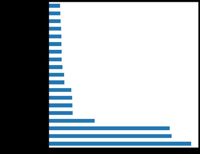
3) Neural Network Feature Importance
3)神经网络特征的重要性
As Keras does not provide a feature importance feature in the documentation i have demonstrated two ways of doing it. Reference is a Stack Over Flow answer.
由于Keras在文档中没有提供功能重要性功能,因此我演示了两种方法。 参考是“堆栈溢出”答案。
from keras.wrappers.scikit_learn import KerasClassifier, KerasRegressor
import eli5
from eli5.sklearn import PermutationImportance
def base_model():
    nn_model = Sequential()    nn_model.add(Dense(64,kernel_regularizer=tf.keras.regularizers.l2(0.001),
                input_dim=46, activation='relu' ))
    nn_model.add(Dropout(rate=0.2))
nn_model.add(Dense(8,kernel_regularizer=tf.keras.regularizers.l2(0.001),
                    activation='relu'))
    nn_model.add(Dropout(rate=0.1))
    nn_model.add(Dense(1, activation='sigmoid'))
    lr_schedule = tf.keras.optimizers.schedules.InverseTimeDecay(
                  0.001,
                  decay_steps=(X_train.shape[0]/32)*50,
                  decay_rate=1,
                  staircase=False)
    def get_optimizer():
        return tf.keras.optimizers.Adam(lr_schedule)
    def get_callbacks():
        return [
            tf.keras.callbacks.EarlyStopping(monitor='val_accuracy',patience=70,restore_best_weights=True)]
    nn_model.compile(loss = "binary_crossentropy",
                  optimizer = get_optimizer(),
                  metrics=['accuracy'])
    return nn_model
my_model = KerasRegressor(build_fn=base_model)
my_model.fit(X_train, y_train, validation_data=(X_test, y_test), epochs=150, batch_size=32,
                    callbacks= get_callbacks(),verbose=0)
perm = PermutationImportance(my_model, random_state=1).fit(X[:500].values,y[:500].values,verbose=False)
eli5.show_weights(perm, feature_names = X.columns.tolist())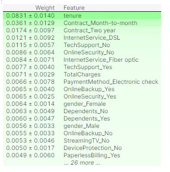
import shap
from tensorflow.keras import Sequential# load JS visualization code to notebook
shap.initjs()# explain the model's predictions using SHAP# (same syntax works for LightGBM, CatBoost, scikit-learn and spark models)
explainer = shap.DeepExplainer(nn_model,data=X[:500].values)
shap_values = explainer.shap_values(X.values)# visualize the first prediction's explanation (use matplotlib=True to avoid Javascript)#shap.force_plot(explainer.expected_value, shap_values[0,:], X.iloc[0,:])
shap.summary_plot(shap_values, X, plot_type="bar")
结论 (Conclusion)
- It can be seen Total charges is the most important feature and rightfully so. The number one reason customers will ‘churn’ if they find the service to be expensive or unaffordable. 可以看出,总收费是最重要的功能,理应如此。 如果客户发现服务昂贵或无法承受,他们将“流失”的第一原因。
- Tenure is also important, the customers who have been using the sevice for a long time or have long time contracts, which are cheaper in general, are less likely to churn. It is interesting to observe that Tenure is listed as more important for neural network model. 任期也很重要,长期使用服务或签订长期合同(通常较便宜)的客户流失的可能性较小。 有趣的是,对于神经网络模型,终身制被列为更重要。
- As observed in the EDA, most customers who are on month to month contracts are more likely to churn. Itcan be hypothesized that the reason is to be attributed to personal reasons of customers to have reservations about long term contracts or higher costs per unit time resulting from monthly contracts. 正如在EDA中观察到的那样,大多数按月签订合同的客户更容易流失。 可以假设该原因归因于客户的个人原因,他们对长期合同有所保留或由于每月合同而导致单位时间的成本较高。
- As seen in EDA, other important features are online security, electronic payment method, fiber optic internet service, tech support. 从EDA中可以看出,其他重要功能包括在线安全性,电子支付方式,光纤互联网服务,技术支持。
- The features which are not important are gender, dependents, partner, streaming TV, backup and device protection. 不重要的功能包括性别,家属,伴侣,流媒体电视,备份和设备保护。
Offers and improving churn rate:
提供和提高流失率:
- Discounts: As the most important feature is total charges, followed by monthly charges, potential churners identified through the modelling should be offered huge discount on next month or months contract. This covers 80 % of the reasons identified for churning. For this modelling, the False Negative Rate should be minimized or Recall should be maximized so that the discounts are sent to maximum of the potential churners. 折扣:由于最重要的功能是总费用,其次是月度费用,因此应在下个月或几个月的合同中为通过模型确定的潜在客户提供巨大的折扣。 这涵盖了确定的搅动原因的80%。 对于此建模,应将误报率最小化或将召回率最大化,以便将折扣发送到最大潜在客户。
- New contract: A six month or four month contract should be implemented. This will encourage the reserved customers who want shorter contracts and will increase their tenure on the service thus making them less likely to churn. 新合同:应执行六个月或四个月的合同。 这将鼓励想要较短合同的保留客户,并增加其服务期限,从而减少他们流失的可能性。
- Online Security: This service should be promoted more and offered complimentary/free for trial periods depending on cost to company. The customers who do not have online security are more likely to churn and thus this offer could be combined with the first one mentioned and discount could only be offered on this. 在线安全:应进一步推广此服务,并根据公司成本免费提供免费试用期。 没有在线安全性的客户更容易流失,因此,此优惠可以与所提到的第一个优惠结合使用,并且只能为此提供优惠。
- Fiber optic: The fiber optic internet is costly and thus should either be promoted to appropriate target audience or better technology can be implemented to cut cost on this service. Ultimately the market research team has to decide the break even point for this service, whether it is profiting as much as the loss of customers it is causing. 光纤:光纤互联网非常昂贵,因此应将其推广给适当的目标受众,或者可以采用更好的技术来削减此服务的成本。 最终,市场研究团队必须决定这项服务的收支平衡点,无论其收益与造成的客户流失一样多。
Another method to quantify the offers to be made is using manually generated features and their effect on the model.
量化报价的另一种方法是使用手动生成的特征及其对模型的影响。
翻译自: https://towardsdatascience.com/churn-prediction-using-neural-networks-and-ml-models-c817aadb7057