进阶篇
目录
模型实用技巧
特征提升
特征抽取
特征筛选
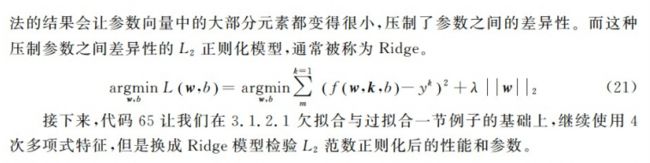
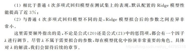
模型正则化
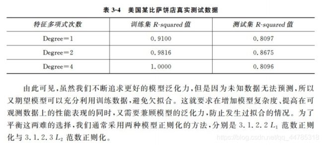
欠拟合与过拟合
L1范数正则化
L2范数正则化
模型检测
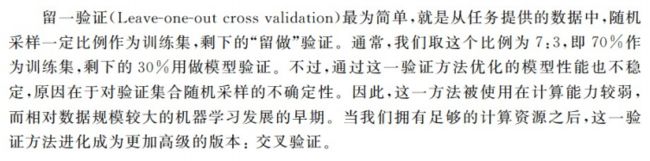
留一验证
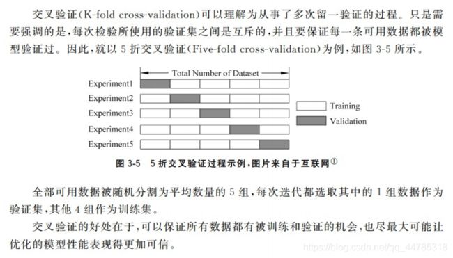
交叉验证
超参数搜索
网格搜索
并行搜索
流行库/模型实践
自然语言处理包(NLTK)
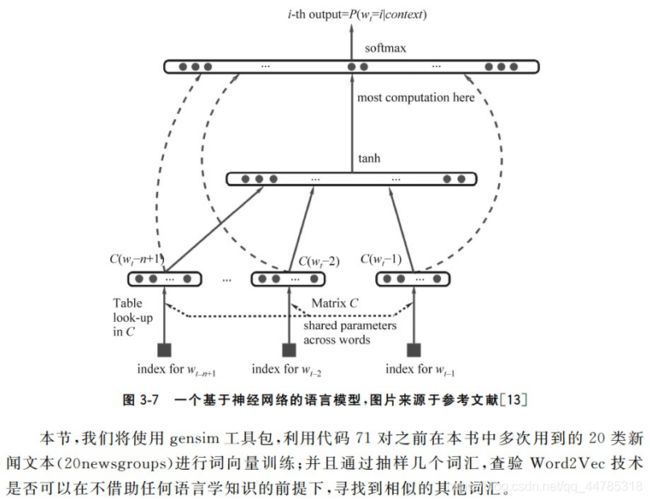
词向量(Word2Vec)技术
XGBoost模型
Tensorflow框架
模型实用技巧
特征提升

特征抽取

DicVectorizer对使用字典存储的数据进行特征抽取与向量化
#定义一组字典列表,用来表示多个数据样本(每个字典代表一个数据样本)
measurements = [{'city':'Dubai','temperature':33.},{'city':'London','temperature':12.},{'city':'San Fransisco','temperature':18.}]
#从 sklearn.feature_extravtion 导入 DictVectorizer
from sklearn.feature_extraction import DictVectorizer
#初始化 DictVectorizer 特征抽取器
vec = DictVectorizer()
#输出转化之后的特征矩阵
print(len(measurements))
print(vec.fit_transform(measurements))
print(vec.fit_transform(measurements).toarray())
#输出各个维度的特征含义
print(vec.get_feature_names())

结果:
3
  (0, 0)	1.0
  (0, 3)	33.0
  (1, 1)	1.0
  (1, 3)	12.0
  (2, 2)	1.0
  (2, 3)	18.0
[[ 1.  0.  0. 33.]
 [ 0.  1.  0. 12.]
 [ 0.  0.  1. 18.]]
['city=Dubai', 'city=London', 'city=San Fransisco', 'temperature']
使用 CountVectorizer 并且不去掉停用词的条件下,对文本特征进行量化的朴素贝叶斯分类性能测试
#从 skearn.datasets 里导入20类新闻文本数据抓取器
from sklearn.datasets import fetch_20newsgroups
from sklearn.model_selection import train_test_split
from sklearn.feature_extraction.text import CountVectorizer
from sklearn.naive_bayes import MultinomialNB
from sklearn.metrics import classification_report

#从互联网上即使下载新闻样本,subset='all'参数代表下载全部近2万条文本存储在变量news中
news = fetch_20newsgroups(subset='all')
#从 sklearn.model_selection 导入 train_test_split 模块用于分割数据集
#对 news 中的数据 data 进行分割,25%的文本用作测试集,75%作为训练集
X_train,X_test,y_train,y_test = train_test_split(news.data,news.target,test_size=0.25,random_state=33)

#从 sklearn.feature_extraction.text 里导入 CountVectorizer
#采用默认的配置对 CountVectorizer 进行初始化(默认配置不去除英文停用词),并且赋值给变量 count_vec
cout_vec = CountVectorizer()

#只使用词频率统计的方式将原始训练和测试文本转化为特征向量
X_count_train = cout_vec.fit_transform(X_train)
X_count_test = cout_vec.transform(X_test)
#从 sklearn.naive_bayes 里导入朴素叶贝斯分类器
#使用默认的配置对分类器进行初始化
mnb_count = MultinomialNB()
#使用朴素叶贝斯分类器,对 CountVectorizer(不去除停用词)后的训练样本进行参数学习
mnb_count.fit(X_count_train,y_train)

#输出模型准确性结果
print("The accuracy of classifying 20newsgroups using Naive Bayes (CountVecorizer without filtering stopwords):",mnb_count.score(X_count_test,y_test))
#将分类预测的结果存储在变量 y_zount_predict 中
y_count_predict = mnb_count.predict(X_count_test)
#从 sklearn.metrics 导入 classification_report
#输出更加详细的其他评价分类性能的指标
print(classification_report(y_test,y_count_predict,target_names=news.target_names))

结果:
The accuracy of classifying 20newsgroups using Naive Bayes (CountVecorizer without filtering stopwords): 0.8397707979626485
                          precision    recall  f1-score   support

             alt.atheism       0.86      0.86      0.86       201
           comp.graphics       0.59      0.86      0.70       250
 comp.os.ms-windows.misc       0.89      0.10      0.17       248
comp.sys.ibm.pc.hardware       0.60      0.88      0.72       240
   comp.sys.mac.hardware       0.93      0.78      0.85       242
          comp.windows.x       0.82      0.84      0.83       263
            misc.forsale       0.91      0.70      0.79       257
               rec.autos       0.89      0.89      0.89       238
         rec.motorcycles       0.98      0.92      0.95       276
      rec.sport.baseball       0.98      0.91      0.95       251
        rec.sport.hockey       0.93      0.99      0.96       233
               sci.crypt       0.86      0.98      0.91       238
         sci.electronics       0.85      0.88      0.86       249
                 sci.med       0.92      0.94      0.93       245
               sci.space       0.89      0.96      0.92       221
  soc.religion.christian       0.78      0.96      0.86       232
      talk.politics.guns       0.88      0.96      0.92       251
   talk.politics.mideast       0.90      0.98      0.94       231
      talk.politics.misc       0.79      0.89      0.84       188
      talk.religion.misc       0.93      0.44      0.60       158

                accuracy                           0.84      4712
               macro avg       0.86      0.84      0.82      4712
            weighted avg       0.86      0.84      0.82      4712
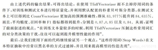
使用 TfidfVectorizer并且不去掉停用词的条件下,对文本特征进行量化的朴素贝叶斯分类性能测试
#从 skearn.datasets 里导入20类新闻文本数据抓取器
from sklearn.datasets import fetch_20newsgroups
from sklearn.model_selection import train_test_split
from sklearn.feature_extraction.text import TfidfVectorizer
from sklearn.naive_bayes import MultinomialNB
from sklearn.metrics import classification_report

#从互联网上即使下载新闻样本,subset='all'参数代表下载全部近2万条文本存储在变量news中
news = fetch_20newsgroups(subset='all')
#从 sklearn.model_selection 导入 train_test_split 模块用于分割数据集
#对 news 中的数据 data 进行分割,25%的文本用作测试集,75%作为训练集
X_train,X_test,y_train,y_test = train_test_split(news.data,news.target,test_size=0.25,random_state=33)

#从 sklearn.feature_extraction.text 里导入 TfidfVectorizer
#采用默认的配置对 TfidfVectorizer 进行初始化(默认配置不去除英文停用词),并且赋值给变量 count_vec
tfidf_vec = TfidfVectorizer()

#只使用词频率统计的方式将原始训练和测试文本转化为特征向量
X_tfidf_train = tfidf_vec.fit_transform(X_train)
X_tfidf_test = tfidf_vec.transform(X_test)
#从 sklearn.naive_bayes 里导入朴素叶贝斯分类器
#使用默认的配置对分类器进行初始化
mnb_tfidf = MultinomialNB()
#使用朴素叶贝斯分类器,对 TfidfVectorizer(不去除停用词)后的训练样本进行参数学习
mnb_tfidf.fit(X_tfidf_train,y_train)

#输出模型准确性结果
print("The accuracy of classifying 20newsgroups using Naive Bayes (TfidfVectorizer without filtering stopwords):",mnb_tfidf.score(X_tfidf_test,y_test))
#将分类预测的结果存储在变量 y_zount_predict 中
y_tfidf_predict = mnb_tfidf.predict(X_tfidf_test)
#从 sklearn.metrics 导入 classification_report
#输出更加详细的其他评价分类性能的指标
print(classification_report(y_test,y_tfidf_predict,target_names=news.target_names))

结果:
The accuracy of classifying 20newsgroups using Naive Bayes (TfidfVectorizer without filtering stopwords): 0.8463497453310697
                          precision    recall  f1-score   support

             alt.atheism       0.84      0.67      0.75       201
           comp.graphics       0.85      0.74      0.79       250
 comp.os.ms-windows.misc       0.82      0.85      0.83       248
comp.sys.ibm.pc.hardware       0.76      0.88      0.82       240
   comp.sys.mac.hardware       0.94      0.84      0.89       242
          comp.windows.x       0.96      0.84      0.89       263
            misc.forsale       0.93      0.69      0.79       257
               rec.autos       0.84      0.92      0.88       238
         rec.motorcycles       0.98      0.92      0.95       276
      rec.sport.baseball       0.96      0.91      0.94       251
        rec.sport.hockey       0.88      0.99      0.93       233
               sci.crypt       0.73      0.98      0.83       238
         sci.electronics       0.91      0.83      0.87       249
                 sci.med       0.97      0.92      0.95       245
               sci.space       0.89      0.96      0.93       221
  soc.religion.christian       0.51      0.97      0.67       232
      talk.politics.guns       0.83      0.96      0.89       251
   talk.politics.mideast       0.92      0.97      0.95       231
      talk.politics.misc       0.98      0.62      0.76       188
      talk.religion.misc       0.93      0.16      0.28       158

                accuracy                           0.85      4712
               macro avg       0.87      0.83      0.83      4712
            weighted avg       0.87      0.85      0.84      4712
特征筛选

#导入 pandas 并且更名为pd
import pandas as pd
from sklearn.model_selection import train_test_split
from sklearn.feature_extraction import DictVectorizer
from sklearn.tree import DecisionTreeClassifier
from sklearn import feature_selection
from sklearn.model_selection import cross_val_score
import numpy as np
import pylab as pl
#从互联网读入titanic 数据
#titanic = pd.read_csv('http://biostat.mc.vanderbilt.edu/wiki/pub/Main/DataSets/titanic.txt')
titanic = pd.read_csv('train.csv')
#分离数据特征与预测目标
y = titanic['Survived']
X = titanic.drop(['Name','Survived'],axis=1)
#对对缺失数据进行填充
X['Age'].fillna(X['Age'].mean(),inplace = True)
X.fillna('UNKNOWN',inplace=True)
#分割数据,依然采用 25% 用于测试
X_train,X_test,y_train,y_test = train_test_split(X,y,test_size=0.25,random_state=33)
#类别型特征向量化
vec = DictVectorizer()
X_train = vec.fit_transform(X_train.to_dict(orient = 'records'))
X_test = vec.transform(X_test.to_dict(orient = 'records'))
#输入处理后特征向量的维度
print("处理后维度:",len(vec.feature_names_))
#使用决策树模型依靠所有特征进行预测,并作性能评估
dt = DecisionTreeClassifier(criterion='entropy')
dt.fit(X_train,y_train)
print("所有特征进行预测:",dt.score(X_test,y_test))
#从 sklearn 导入特征筛选器
#筛选前 20% 的特征,使用相同配置的决策树模型进行预测,并且评估性能
fs = feature_selection.SelectPercentile(feature_selection.chi2,percentile=20)
X_train_fs = fs.fit_transform(X_train,y_train)
dt.fit(X_train_fs,y_train)
X_test_fs = fs.transform(X_test)
print("选择前20%的特征进行预测:",dt.score(X_test_fs,y_test))
#通过交叉验证的方法,按照固定间隔的百分比筛选特征,并作图展示性能随特征筛选比例的变化
percentiles = range(1,100,2)
results = []
for i in percentiles:
fs = feature_selection.SelectPercentile(feature_selection.chi2,percentile=i)
X_train_fs = fs.fit_transform(X_train,y_train)
#dt为需要使用交叉验证的算法,输入样本,样本标签,cv为交叉验证折数或可迭代的次数
scores = cross_val_score(dt,X_train_fs,y_train,cv=5)
#results 为需要被添加的值的数组,scores.mean为添加的值
results = np.append(results,scores.mean())
print("选择 从前百分之 1到99 间隔为2的特征分别进行预测")
print(results)
pl.plot(percentiles,results)
pl.xlabel("percentiles of features")
pl.ylabel('accuracy')
pl.show()
#使用最佳筛选后的特征,利用相同配置的模型在测试集上进行性能评估
fs = feature_selection.SelectPercentile(feature_selection.chi2,percentile=60)
X_train_fs = fs.fit_transform(X_train,y_train)
dt.fit(X_train_fs,y_train)
X_test_fs = fs.transform(X_test)
print(dt.score(X_test_fs,y_test))
结果:
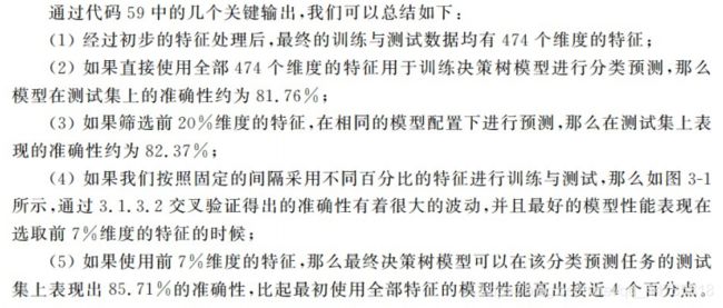
处理后维度: 684
所有特征进行预测: 0.820627802690583
选择前20%的特征进行预测: 0.8385650224215246
选择 从前百分之 1到99 间隔为2的特征分别进行预测
[0.74998317 0.74250926 0.74849063 0.74851307 0.74548311 0.76349456
0.75897206 0.7574683 0.75597576 0.76196835 0.75898328 0.78443497
0.76045337 0.7574683 0.75594209 0.77692739 0.75897206 0.7739311
0.76794973 0.77993491 0.76645719 0.76948715 0.76498709 0.7769835
0.7754573 0.76647963 0.77843115 0.77248345 0.78594995 0.78743126
0.78146112 0.77847604 0.77696106 0.77846482 0.77841993 0.77847604
0.78446863 0.7754573 0.77693862 0.77243856 0.78293121 0.77544608
0.77840871 0.77550219 0.77999102 0.77399843 0.78296487 0.7784536
0.7754573 0.78294243]
0.8116591928251121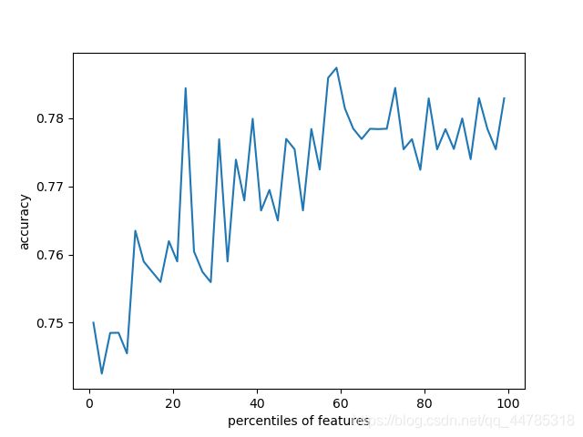
模型正则化
欠拟合与过拟合

from sklearn.linear_model import LinearRegression
import numpy as np
import matplotlib.pylab as plt
#输入训练样本的特征以及目标值,分别存储在变量 X_train 与 y_train 之中
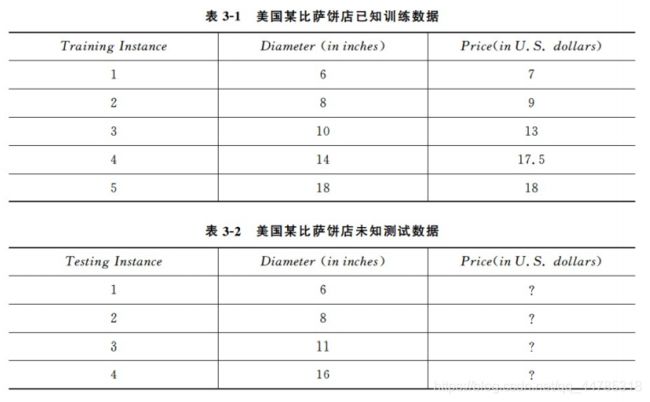
X_train = [[6],[8],[10],[14],[18]]
y_train = [[7],[9],[13],[17.5],[18]]
#从 sklearn.linear_model 中导入 LinearRegression
#使用默认配置初始化线性回归模型
regressor = LinearRegression()
#直接以披萨的直径作为特征训练模型
regressor.fit(X_train,y_train)
#训练完毕
#导入 numpy 并且重命名为 np
#在 x轴上从0至25均匀采样100个数据点
xx = np.linspace(0,26,100)
xx = xx.reshape(xx.shape[0],1) #改变数组的维数样式
#以上述100个数据点作为基准,预测回归直线
yy = regressor.predict(xx)
#对回归预测到的直线进行作图
#绘制数据集点
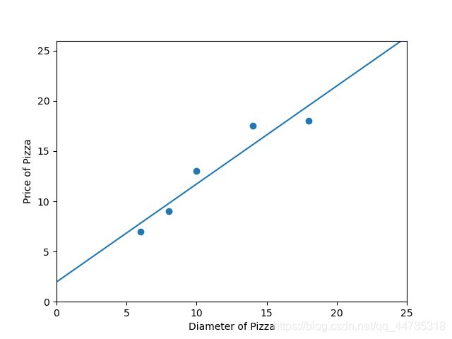
plt.scatter(X_train,y_train)
#在同一张图中画训练完的回归线
plt1, = plt.plot(xx,yy,label ='Degree=1')
plt.axis([0,25,0,26]) #坐标大小为 x、y轴从0到25
plt.xlabel('Diameter of Pizza')
plt.ylabel('Price of Pizza')
plt.legend(handles = [plt1])
plt.show()
#输出线性回归模型在训练样本上的R-squared值
print("The R-squared value of Linear Regressor performing on the training data is",regressor.score(X_train,y_train))
结果:
The R-squared value of Linear Regressor performing on the training data is 0.9100015964240102
from sklearn.preprocessing import PolynomialFeatures
from sklearn.linear_model import LinearRegression
import numpy as np
import matplotlib.pyplot as plt
#输入训练样本的特征以及目标值,分别存储在变量 X_train 与 y_train 之中
X_train = [[6],[8],[10],[14],[18]]
y_train = [[7],[9],[13],[17.5],[18]]
#以线性回归器为基础,初始化回归模型。尽管特征的维度有提高,但是模型基础仍然是线性模型
regressor_poly2 = LinearRegression()
#从 sklearn.linear_model 中导入 LinearRegression
#使用默认配置初始化线性回归模型
regressor = LinearRegression()
#从 sklearn.preproessing 中导入多项式特征产生器
#使用 PolynorminalFeatures(degress = 2)映射出2次多项式特征,存储在变量 X_train_poly2中
poly2 = PolynomialFeatures(degree=2)
X_train_poly2 = poly2.fit_transform(X_train)
#对2次多项式回归模型进行训练
regressor_poly2.fit(X_train_poly2,y_train)
#直接以披萨的直径作为特征训练模型
regressor.fit(X_train,y_train)
#从新映射绘图用 x 轴采样数据
xx = np.linspace(0,26,100)
xx = xx.reshape(xx.shape[0],1)
xx_poly2 = poly2.transform(xx)
#以上述100个数据点作为基准,预测回归直线
yy = regressor.predict(xx)
#使用2次多项式回归模型对应x轴采样数据进行回归预测
yy_poly2 = regressor_poly2.predict(xx_poly2)
#分别对训练数据点、线型回归直线、2次多项式回归曲线进行作图
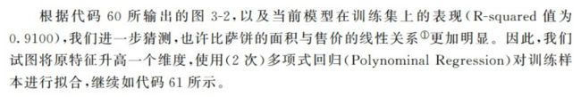
plt.scatter(X_train,y_train)
plt1, = plt.plot(xx,yy,label = 'Degree=1')
plt2, = plt.plot(xx,yy_poly2,label = 'Degree=2')
plt.axis([0,25,0,25])
plt.xlabel("Diameter of Pizza")
plt.ylabel("Price of Pizza")
plt.legend(handles = [plt1,plt2])
plt.show()
#输出线性回归模型在训练样本上的R-squared值
print("The R-squared value of Linear Regressor performing on the training data is",regressor.score(X_train,y_train))
#输出2次多项式回归模型在训练样本上的R_squared值
print("The R-squared value of Polynorminak Regressor (Degree=2) performing on the training data is",regressor_poly2.score(X_train_poly2,y_train))
结果:
The R-squared value of Linear Regressor performing on the training data is 0.9100015964240102
The R-squared value of Polynorminak Regressor (Degree=2) performing on the training data is 0.9816421639597427
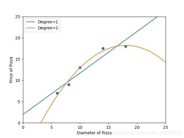
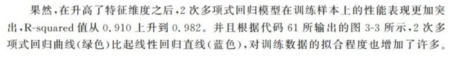
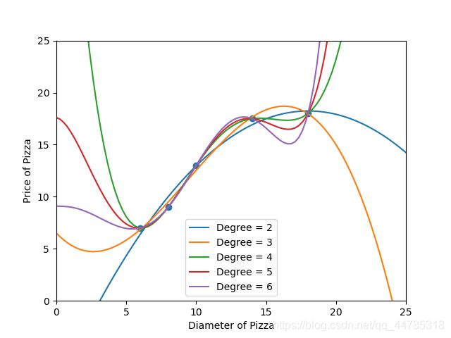
由此进一步升高特征维度
from sklearn.preprocessing import PolynomialFeatures
from sklearn.linear_model import LinearRegression
import numpy as np
import matplotlib.pyplot as plt

#输入训练样本的特征以及目标值,分别存储在变量 X_train 与 y_train 之中
X_train = [[6],[8],[10],[14],[18]]
y_train = [[7],[9],[13],[17.5],[18]]

#从新映射绘图用 x 轴采样数据
xx = np.linspace(0,26,100)
xx = xx.reshape(xx.shape[0],1)

range = range(2,7)

plt.scatter(X_train,y_train)
plt.axis([0,25,0,25])
plt.xlabel("Diameter of Pizza")
plt.ylabel("Price of Pizza")

pltInfo=[]
for i in range:
    #准备工作
    poly = "poly"+str(i)
    plts = "plt" + str(i)
    Degree = "Degree = "+str(i)
    regressor_poly = "regressor_poly"+str(i)
    xx_poly = "xx_poly" + str(i)
    yy_poly = "yy_poly" + str(i)

    # 从 sklearn.preproessing 中导入多项式特征产生器
    # 使用 PolynorminalFeatures(degress = i)映射出第i次多项式特征,存储在变量 X_train_poly中
    poly = PolynomialFeatures(degree=i)
    X_train_poly = poly.fit_transform(X_train)
    # 以线性回归器为基础,初始化回归模型。尽管特征的维度有提高,但是模型基础仍然是线性模型
    regressor_poly = LinearRegression()
    # 对i次多项式回归模型进行训练
    regressor_poly.fit(X_train_poly,y_train)

    #将xx的数据作为测试集
    xx_poly = poly.transform(xx)
    #训练xx_poly集,并将结果存储到yy_poly
    yy_poly = regressor_poly.predict(xx_poly)

    #将每次作图信息存入一个列表中
    pltInfo.append(plts)
    #定义每一个作图信息
    pltInfo[i-2], =plt.plot(xx,yy_poly,label = Degree)
    #应用作图信息
    plt.legend(handles=pltInfo)
    # 输出i次多项式回归模型在训练样本上的R_squared值
    print("The R-squared value of Polynorminak Regressor (",Degree,") performing on the training data is",regressor_poly.score(X_train_poly, y_train))

plt.show()

结果:
The R-squared value of Polynorminak Regressor ( Degree = 2 ) performing on the training data is 0.9816421639597427
The R-squared value of Polynorminak Regressor ( Degree = 3 ) performing on the training data is 0.9947351016429964
The R-squared value of Polynorminak Regressor ( Degree = 4 ) performing on the training data is 1.0
The R-squared value of Polynorminak Regressor ( Degree = 5 ) performing on the training data is 1.0
The R-squared value of Polynorminak Regressor ( Degree = 6 ) performing on the training data is 1.0
from sklearn.preprocessing import PolynomialFeatures
from sklearn.linear_model import LinearRegression
import numpy as np
import matplotlib.pyplot as plt
#输入训练样本的特征以及目标值,分别存储在变量 X_train 与 y_train 之中
X_train = [[6],[8],[10],[14],[18]]
y_train = [[7],[9],[13],[17.5],[18]]
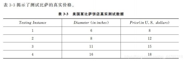
#准备测试数据
X_test = [[6],[8],[11],[16]]
y_test = [[8],[12],[15],[18]]
#使用测试数据对线性回归模型的性能进行评估
regressor = LinearRegression()
regressor.fit(X_train,y_train)
print(regressor.score(X_test,y_test))
#使用测试数据对2次多项式回归模型的性能进行评估
poly2 = PolynomialFeatures(degree=2)
X_train_poly2 = poly2.fit_transform(X_train)
regressor_poly2 = LinearRegression()
regressor_poly2.fit(X_train_poly2,y_train)
X_test_poly2 = poly2.transform(X_test)
print(regressor_poly2.score(X_test_poly2,y_test))
#使用测试数据对4次多项式回归模型的性能进行评估
poly4 = PolynomialFeatures(degree=4)
X_train_poly4 = poly4.fit_transform(X_train)
regressor_poly4 = LinearRegression()
regressor_poly4.fit(X_train_poly4,y_train)
X_test_poly4 = poly4.transform(X_test)
print(regressor_poly4.score(X_test_poly4,y_test))
结果:
0.809726797707665
0.8675443656345054
0.8095880795856146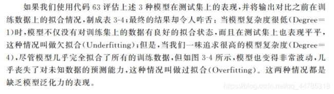
L1范数正则化
from sklearn.preprocessing import PolynomialFeatures
from sklearn.linear_model import LinearRegression
import numpy as np
import matplotlib.pyplot as plt
from sklearn.linear_model import Lasso

#输入训练样本的特征以及目标值,分别存储在变量 X_train 与 y_train 之中
X_train = [[6],[8],[10],[14],[18]]
y_train = [[7],[9],[13],[17.5],[18]]

#准备测试数据
X_test = [[6],[8],[11],[16]]
y_test = [[8],[12],[15],[18]]

#使用测试数据对4次多项式回归模型的性能进行评估
poly4 = PolynomialFeatures(degree=4)
X_train_poly4 = poly4.fit_transform(X_train)

regressor_poly4 = LinearRegression()
regressor_poly4.fit(X_train_poly4,y_train)

X_test_poly4 = poly4.transform(X_test)
print("普通4次多项式",regressor_poly4.score(X_test_poly4,y_test))
#普通4次多项式回归模型的参数列表
print(regressor_poly4.coef_)

#从sklearn.linear_model 中导入Lasso
lasso_poly4 = Lasso()
#从使用 Lasso 对4次多项式特征进行拟合
lasso_poly4.fit(X_train_poly4,y_train)

#对 Lasso模型在测试样本上的回归性能进行评估
print('Lasso模型:',lasso_poly4.score(X_train_poly4,y_train))
print(lasso_poly4.coef_)

结果:
普通4次多项式 0.8095880795856146
[[ 0.00000000e+00 -2.51739583e+01  3.68906250e+00 -2.12760417e-01
   4.29687500e-03]]
Lasso模型: 0.9940832798380284
[ 0.00000000e+00  0.00000000e+00  1.17900534e-01  5.42646770e-05
 -2.23027128e-04]
L2范数正则化

from sklearn.preprocessing import PolynomialFeatures
from sklearn.linear_model import LinearRegression
import numpy as np
import matplotlib.pyplot as plt
from sklearn.linear_model import Lasso
from sklearn.linear_model import Ridge

#输入训练样本的特征以及目标值,分别存储在变量 X_train 与 y_train 之中
X_train = [[6],[8],[10],[14],[18]]
y_train = [[7],[9],[13],[17.5],[18]]

#准备测试数据
X_test = [[6],[8],[11],[16]]
y_test = [[8],[12],[15],[18]]

#使用测试数据对4次多项式回归模型的性能进行评估
poly4 = PolynomialFeatures(degree=4)
X_train_poly4 = poly4.fit_transform(X_train)

regressor_poly4 = LinearRegression()
regressor_poly4.fit(X_train_poly4,y_train)

X_test_poly4 = poly4.transform(X_test)
print("普通4次多项式",regressor_poly4.score(X_test_poly4,y_test))
#普通4次多项式回归模型的参数列表
print(regressor_poly4.coef_)
#输出上述这些参数的平方和,验证参数之间的巨大差异
print("普通4次参数平方和:",np.sum(regressor_poly4.coef_ ** 2))
print("---"*20)
#从 sklearn.linear_model 导入 Ridge
ridge_poly4 = Ridge()
#使用 Ridge 模型对4次多项式特征进行拟合
ridge_poly4.fit(X_train_poly4,y_train)
#输出Ridge模型在测试样本上的回归性能
print(ridge_poly4.score(X_test_poly4,y_test))
#输出 Ridge 模型的参数列表,观察参数差异
print(ridge_poly4.coef_)
#计算 Ridge 模型拟合后参数的平方和
print("Ridge 模型平方和:",np.sum(ridge_poly4.coef_ ** 2))
print("---"*20)
#从sklearn.linear_model 中导入Lasso
lasso_poly4 = Lasso()
#从使用 Lasso 对4次多项式特征进行拟合
lasso_poly4.fit(X_train_poly4,y_train)
#对 Lasso模型在测试样本上的回归性能进行评估
print('Lasso模型:',lasso_poly4.score(X_train_poly4,y_train))
print('Lasso模型平方和:',np.sum(lasso_poly4.coef_ ** 2))

结果:
普通4次多项式 0.8095880795856146
[[ 0.00000000e+00 -2.51739583e+01  3.68906250e+00 -2.12760417e-01
   4.29687500e-03]]
普通4次参数平方和: 647.3826456916975
------------------------------------------------------------
0.8374201759366509
[[ 0.         -0.00492536  0.12439632 -0.00046471 -0.00021205]]
Ridge 模型平方和: 0.015498965203562037
------------------------------------------------------------
Lasso模型: 0.9940832798380284
Lasso模型平方和: 0.01390058867089999
模型检测

留一验证
交叉验证
超参数搜索

网格搜索

from sklearn.datasets import fetch_20newsgroups
import numpy as np
from sklearn.model_selection import train_test_split
from sklearn.svm import SVC
from sklearn.feature_extraction.text import TfidfVectorizer
from sklearn.pipeline import Pipeline
from  sklearn.model_selection import GridSearchCV

#从sklearn,datasets 中导入20类新闻文本抓取器
#导入 numpy,并且重命名为np

#使用新闻抓取器从互联网上下载所有数据,并且存储在变量news中
news = fetch_20newsgroups(subset="all")
#sklearn.model_selection 导入 train_test_split 用来分割数据
#对前 3000 条新闻文本进行数据分割,25%文本用于未来测试
X_train,X_test,y_train,y_test = train_test_split(news.data[:3000],news.target[:3000],test_size=0.25,random_state=33)

#导入支持向量机(分类)模型
#导入 TfidfVectorizer 文本抽取器
#导入 Pipeline

#使用 Pipeline 简化系统搭建流程,将文本抽取与分类器模型串联起来
clf = Pipeline([('vect',TfidfVectorizer(stop_words='english',analyzer='word')),('svc',SVC())])

#这里需要实验的2个超参数的个数分别是 4、3,svc_gamma的参数共用10^-2,10^--1...这样我们一共有12中的超参数组合,12个不同参数下的模型
parameters = {'svc__gamma':np.logspace(-2,1,4),'svc__C':np.logspace(-1,1,3)}

#从 sklearn.model_selection 中导入网格搜索模块 GridSearchCV
#将12组参数组合以及初始化的Pipline包括 3折交叉验证的要求全部告知 GridSearchCV。请大家务必注意 refit=True 这样一个设定
gs = GridSearchCV(clf,parameters,verbose=2,refit=True,cv = 3)

#执行单线程网格搜索
gs.fit(X_train,y_train)
print(gs.best_params_,gs.best_score_)

#输出最佳模型在测试集上的准确性
print(gs.score(X_test,y_test))

结果:
[Parallel(n_jobs=1)]: Using backend SequentialBackend with 1 concurrent workers.
Fitting 3 folds for each of 12 candidates, totalling 36 fits
[CV] svc__C=0.1, svc__gamma=0.01 .....................................
[CV] ...................... svc__C=0.1, svc__gamma=0.01, total=   4.2s
[CV] svc__C=0.1, svc__gamma=0.01 .....................................
[Parallel(n_jobs=1)]: Done   1 out of   1 | elapsed:    4.1s remaining:    0.0s
[CV] ...................... svc__C=0.1, svc__gamma=0.01, total=   4.2s
[CV] svc__C=0.1, svc__gamma=0.01 .....................................
[CV] ...................... svc__C=0.1, svc__gamma=0.01, total=   4.2s
[CV] svc__C=0.1, svc__gamma=0.1 ......................................
[CV] ....................... svc__C=0.1, svc__gamma=0.1, total=   4.2s
[CV] svc__C=0.1, svc__gamma=0.1 ......................................
[CV] ....................... svc__C=0.1, svc__gamma=0.1, total=   4.2s
[CV] svc__C=0.1, svc__gamma=0.1 ......................................
[CV] ....................... svc__C=0.1, svc__gamma=0.1, total=   4.2s
[CV] svc__C=0.1, svc__gamma=1.0 ......................................
[CV] ....................... svc__C=0.1, svc__gamma=1.0, total=   4.2s
[CV] svc__C=0.1, svc__gamma=1.0 ......................................
[CV] ....................... svc__C=0.1, svc__gamma=1.0, total=   4.3s
[CV] svc__C=0.1, svc__gamma=1.0 ......................................
[CV] ....................... svc__C=0.1, svc__gamma=1.0, total=   4.3s
[CV] svc__C=0.1, svc__gamma=10.0 .....................................
[CV] ...................... svc__C=0.1, svc__gamma=10.0, total=   4.2s
[CV] svc__C=0.1, svc__gamma=10.0 .....................................
[CV] ...................... svc__C=0.1, svc__gamma=10.0, total=   4.3s
[CV] svc__C=0.1, svc__gamma=10.0 .....................................
[CV] ...................... svc__C=0.1, svc__gamma=10.0, total=   4.3s
[CV] svc__C=1.0, svc__gamma=0.01 .....................................
[CV] ...................... svc__C=1.0, svc__gamma=0.01, total=   4.2s
[CV] svc__C=1.0, svc__gamma=0.01 .....................................
[CV] ...................... svc__C=1.0, svc__gamma=0.01, total=   4.2s
[CV] svc__C=1.0, svc__gamma=0.01 .....................................
[CV] ...................... svc__C=1.0, svc__gamma=0.01, total=   4.2s
[CV] svc__C=1.0, svc__gamma=0.1 ......................................
[CV] ....................... svc__C=1.0, svc__gamma=0.1, total=   4.2s
[CV] svc__C=1.0, svc__gamma=0.1 ......................................
[CV] ....................... svc__C=1.0, svc__gamma=0.1, total=   4.2s
[CV] svc__C=1.0, svc__gamma=0.1 ......................................
[CV] ....................... svc__C=1.0, svc__gamma=0.1, total=   4.2s
[CV] svc__C=1.0, svc__gamma=1.0 ......................................
[CV] ....................... svc__C=1.0, svc__gamma=1.0, total=   4.3s
[CV] svc__C=1.0, svc__gamma=1.0 ......................................
[CV] ....................... svc__C=1.0, svc__gamma=1.0, total=   4.3s
[CV] svc__C=1.0, svc__gamma=1.0 ......................................
[CV] ....................... svc__C=1.0, svc__gamma=1.0, total=   4.3s
[CV] svc__C=1.0, svc__gamma=10.0 .....................................
[CV] ...................... svc__C=1.0, svc__gamma=10.0, total=   4.3s
[CV] svc__C=1.0, svc__gamma=10.0 .....................................
[CV] ...................... svc__C=1.0, svc__gamma=10.0, total=   4.3s
[CV] svc__C=1.0, svc__gamma=10.0 .....................................
[CV] ...................... svc__C=1.0, svc__gamma=10.0, total=   4.4s
[CV] svc__C=10.0, svc__gamma=0.01 ....................................
[CV] ..................... svc__C=10.0, svc__gamma=0.01, total=   4.1s
[CV] svc__C=10.0, svc__gamma=0.01 ....................................
[CV] ..................... svc__C=10.0, svc__gamma=0.01, total=   4.2s
[CV] svc__C=10.0, svc__gamma=0.01 ....................................
[CV] ..................... svc__C=10.0, svc__gamma=0.01, total=   4.2s
[CV] svc__C=10.0, svc__gamma=0.1 .....................................
[CV] ...................... svc__C=10.0, svc__gamma=0.1, total=   4.2s
[CV] svc__C=10.0, svc__gamma=0.1 .....................................
[CV] ...................... svc__C=10.0, svc__gamma=0.1, total=   4.2s
[CV] svc__C=10.0, svc__gamma=0.1 .....................................
[CV] ...................... svc__C=10.0, svc__gamma=0.1, total=   4.3s
[CV] svc__C=10.0, svc__gamma=1.0 .....................................
[CV] ...................... svc__C=10.0, svc__gamma=1.0, total=   4.3s
[CV] svc__C=10.0, svc__gamma=1.0 .....................................
[CV] ...................... svc__C=10.0, svc__gamma=1.0, total=   4.3s
[CV] svc__C=10.0, svc__gamma=1.0 .....................................
[CV] ...................... svc__C=10.0, svc__gamma=1.0, total=   4.3s
[CV] svc__C=10.0, svc__gamma=10.0 ....................................
[CV] ..................... svc__C=10.0, svc__gamma=10.0, total=   4.3s
[CV] svc__C=10.0, svc__gamma=10.0 ....................................
[CV] ..................... svc__C=10.0, svc__gamma=10.0, total=   4.4s
[CV] svc__C=10.0, svc__gamma=10.0 ....................................
[CV] ..................... svc__C=10.0, svc__gamma=10.0, total=   4.4s
[Parallel(n_jobs=1)]: Done  36 out of  36 | elapsed:  2.6min finished
{'svc__C': 10.0, 'svc__gamma': 0.1} 0.7888888888888889
0.8226666666666667


并行搜索
from sklearn.datasets import fetch_20newsgroups
import numpy as np
from sklearn.model_selection import train_test_split
from sklearn.svm import SVC
from sklearn.feature_extraction.text import TfidfVectorizer
from sklearn.pipeline import Pipeline
from  sklearn.model_selection import GridSearchCV

#从sklearn,datasets 中导入20类新闻文本抓取器
#导入 numpy,并且重命名为np

#使用新闻抓取器从互联网上下载所有数据,并且存储在变量news中
news = fetch_20newsgroups(subset="all")
#sklearn.model_selection 导入 train_test_split 用来分割数据
#对前 3000 条新闻文本进行数据分割,25%文本用于未来测试
X_train,X_test,y_train,y_test = train_test_split(news.data[:3000],news.target[:3000],test_size=0.25,random_state=33)

#导入支持向量机(分类)模型
#导入 TfidfVectorizer 文本抽取器
#导入 Pipeline

#使用 Pipeline 简化系统搭建流程,将文本抽取与分类器模型串联起来
clf = Pipeline([('vect',TfidfVectorizer(stop_words='english',analyzer='word')),('svc',SVC())])

#这里需要实验的2个超参数的个数分别是 4、3,svc_gamma的参数共用10^-2,10^--1...这样我们一共有12中的超参数组合,12个不同参数下的模型
#logspace为生成等比数列 默认底数为10(-2,1,4)指从幂-2 -1 0 1 共4个
parameters = {'svc__gamma':np.logspace(-2,1,4),'svc__C':np.logspace(-1,1,3)}

#从 sklearn.model_selection 中导入网格搜索模块 GridSearchCV
#将12组参数组合以及初始化的Pipline包括 3折交叉验证的要求全部告知 GridSearchCV。请大家务必注意 refit=True 这样一个设定
#初始化配置并行网格搜索,n_jobs = -1代表使用该计算机全部的CPU
gs = GridSearchCV(clf,parameters,verbose=2,refit=True,cv = 3,n_jobs=-1)

#执行多线程并行网格搜索
gs.fit(X_train,y_train)
print(gs.best_params_,gs.best_score_)

#输出最佳模型在测试集上的准确性
print(gs.score(X_test,y_test))

结果:
D:\anaconda3\envs\pythonProject1\python.exe D:/PycharmProjects/test1/1.py
Fitting 3 folds for each of 12 candidates, totalling 36 fits
[Parallel(n_jobs=-1)]: Using backend LokyBackend with 12 concurrent workers.
[CV] svc__C=0.1, svc__gamma=0.01 .....................................
[CV] svc__C=0.1, svc__gamma=0.01 .....................................
[CV] svc__C=0.1, svc__gamma=0.01 .....................................
[CV] svc__C=0.1, svc__gamma=0.1 ......................................
[CV] svc__C=0.1, svc__gamma=0.1 ......................................
[CV] svc__C=0.1, svc__gamma=0.1 ......................................
[CV] svc__C=0.1, svc__gamma=1.0 ......................................
[CV] svc__C=0.1, svc__gamma=10.0 .....................................
[CV] svc__C=0.1, svc__gamma=10.0 .....................................
[CV] svc__C=0.1, svc__gamma=1.0 ......................................
[CV] svc__C=0.1, svc__gamma=1.0 ......................................
[CV] svc__C=0.1, svc__gamma=10.0 .....................................
[CV] ...................... svc__C=0.1, svc__gamma=0.01, total=   5.9s
[CV] ...................... svc__C=0.1, svc__gamma=0.01, total=   5.9s
[CV] svc__C=1.0, svc__gamma=0.01 .....................................
[CV] svc__C=1.0, svc__gamma=0.01 .....................................
[CV] ....................... svc__C=0.1, svc__gamma=0.1, total=   5.9s
[CV] ...................... svc__C=0.1, svc__gamma=0.01, total=   6.0s
[CV] ....................... svc__C=0.1, svc__gamma=0.1, total=   5.9s
[CV] svc__C=1.0, svc__gamma=0.01 .....................................
[CV] svc__C=1.0, svc__gamma=0.1 ......................................
[CV] svc__C=1.0, svc__gamma=0.1 ......................................
[CV] ....................... svc__C=0.1, svc__gamma=0.1, total=   6.0s
[CV] ....................... svc__C=0.1, svc__gamma=1.0, total=   6.0s
[CV] svc__C=1.0, svc__gamma=0.1 ......................................
[CV] svc__C=1.0, svc__gamma=1.0 ......................................
[CV] ...................... svc__C=0.1, svc__gamma=10.0, total=   6.0s
[CV] svc__C=1.0, svc__gamma=1.0 ......................................
[CV] ...................... svc__C=0.1, svc__gamma=10.0, total=   7.7s
[CV] svc__C=1.0, svc__gamma=1.0 ......................................
[CV] ...................... svc__C=0.1, svc__gamma=10.0, total=   7.8s
[CV] svc__C=1.0, svc__gamma=10.0 .....................................
[CV] ....................... svc__C=0.1, svc__gamma=1.0, total=   8.1s
[CV] svc__C=1.0, svc__gamma=10.0 .....................................
[CV] ....................... svc__C=0.1, svc__gamma=1.0, total=   8.9s
[CV] svc__C=1.0, svc__gamma=10.0 .....................................
[CV] ...................... svc__C=1.0, svc__gamma=0.01, total=   5.9s
[CV] svc__C=10.0, svc__gamma=0.01 ....................................
[CV] ....................... svc__C=1.0, svc__gamma=0.1, total=   6.3s
[CV] svc__C=10.0, svc__gamma=0.01 ....................................
[CV] ....................... svc__C=1.0, svc__gamma=1.0, total=   6.3s
[CV] svc__C=10.0, svc__gamma=0.01 ....................................
[CV] ....................... svc__C=1.0, svc__gamma=1.0, total=   6.4s
[CV] svc__C=10.0, svc__gamma=0.1 .....................................
[CV] ...................... svc__C=1.0, svc__gamma=0.01, total=   7.5s
[CV] svc__C=10.0, svc__gamma=0.1 .....................................
[CV] ....................... svc__C=1.0, svc__gamma=0.1, total=   7.6s
[CV] ...................... svc__C=1.0, svc__gamma=0.01, total=   7.7s
[CV] ....................... svc__C=1.0, svc__gamma=0.1, total=   7.5s
[CV] svc__C=10.0, svc__gamma=0.1 .....................................
[CV] svc__C=10.0, svc__gamma=1.0 .....................................
[CV] svc__C=10.0, svc__gamma=1.0 .....................................
[CV] ...................... svc__C=1.0, svc__gamma=10.0, total=   6.0s
[CV] svc__C=10.0, svc__gamma=1.0 .....................................
[CV] ....................... svc__C=1.0, svc__gamma=1.0, total=   6.7s
[CV] svc__C=10.0, svc__gamma=10.0 ....................................
[CV] ...................... svc__C=1.0, svc__gamma=10.0, total=   7.6s
[CV] svc__C=10.0, svc__gamma=10.0 ....................................
[CV] ...................... svc__C=1.0, svc__gamma=10.0, total=   7.3s
[CV] svc__C=10.0, svc__gamma=10.0 ....................................
[CV] ..................... svc__C=10.0, svc__gamma=0.01, total=   6.4s
[CV] ..................... svc__C=10.0, svc__gamma=0.01, total=   6.0s
[CV] ..................... svc__C=10.0, svc__gamma=0.01, total=   6.4s
[CV] ...................... svc__C=10.0, svc__gamma=0.1, total=   6.4s
[CV] ...................... svc__C=10.0, svc__gamma=1.0, total=   6.0s
[CV] ...................... svc__C=10.0, svc__gamma=0.1, total=   6.9s
[CV] ...................... svc__C=10.0, svc__gamma=1.0, total=   6.8s
[Parallel(n_jobs=-1)]: Done  32 out of  36 | elapsed:   22.9s remaining:    2.8s
[CV] ...................... svc__C=10.0, svc__gamma=0.1, total=   6.9s
[CV] ...................... svc__C=10.0, svc__gamma=1.0, total=   6.9s
[CV] ..................... svc__C=10.0, svc__gamma=10.0, total=   5.9s
[CV] ..................... svc__C=10.0, svc__gamma=10.0, total=   5.7s
[CV] ..................... svc__C=10.0, svc__gamma=10.0, total=   5.5s
[Parallel(n_jobs=-1)]: Done  36 out of  36 | elapsed:   24.4s finished
{'svc__C': 10.0, 'svc__gamma': 0.1} 0.7888888888888889
0.8226666666666667

流行库/模型实践
自然语言处理包(NLTK)
from sklearn.feature_extraction.text import CountVectorizer

#将上述两个句子以字符串的数据类型分别存储在变量 sent1 与 sent2中
sent1 = "The cat is walking in the bedroom."
sent2 = "A dog was running access the kitchen."

#从 sklearn.feature_extraction.text 中导入 CountVectorizer
count_vec = CountVectorizer()

sentences = [sent1,sent2]

#输出特征向量化后的表示
print(count_vec.fit_transform(sentences).toarray())
#输出向量各个维度的特征含义
print(count_vec.get_feature_names())

结果:
[[0 1 1 0 1 1 0 0 2 1 0]
 [1 0 0 1 0 0 1 1 1 0 1]]
['access', 'bedroom', 'cat', 'dog', 'in', 'is', 'kitchen', 'running', 'the', 'walking', 'was']

from sklearn.feature_extraction.text import CountVectorizer
import nltk

#将上述两个句子以字符串的数据类型分别存储在变量 sent1 与 sent2中
sent1 = "The cat is walking in the bedroom."
sent2 = "A dog was running access the kitchen."
sentences = [sent1,sent2]

#从 sklearn.feature_extraction.text 中导入 CountVectorizer
count_vec = CountVectorizer()
#输出特征向量化后的表示
print(count_vec.fit_transform(sentences).toarray())
#输出向量各个维度的特征含义
print(count_vec.get_feature_names())
print("--"*40)

#导入 nltk
#对句子进行词汇分割和正规化,有些情况如aren't 需要分割为 are 和 n't ;或者 I'm要分割为I和'm
tokens_1 = nltk.word_tokenize(sent1)
print(tokens_1)
tokens_2 = nltk.word_tokenize(sent2)
print(tokens_2)
print("--"*40)

#整理两句的词表,并且按照ASCLL的排序输出
#set为去重
vocab_1 = sorted(set(tokens_1))
print(vocab_1)
vocab_2 = sorted(set(tokens_2))
print(vocab_2)
print("--"*40)

#初始化 stemmer 寻找各个词汇最原始的词根
stemmer = nltk.stem.PorterStemmer()
stem_1 = [stemmer.stem(t) for t in tokens_1]
print(stem_1)
stem_2 = [stemmer.stem(t) for t in tokens_2]
print(stem_2)
print("--"*40)

#初始化词性标注器,对每个词汇进行标注
pos_tag_1 = nltk.tag.pos_tag(tokens_1)
print(pos_tag_1)
pos_tag_2 = nltk.tag.pos_tag(tokens_2)
print(pos_tag_2)

结果:
[[0 1 1 0 1 1 0 0 2 1 0]
 [1 0 0 1 0 0 1 1 1 0 1]]
['access', 'bedroom', 'cat', 'dog', 'in', 'is', 'kitchen', 'running', 'the', 'walking', 'was']
--------------------------------------------------------------------------------
['The', 'cat', 'is', 'walking', 'in', 'the', 'bedroom', '.']
['A', 'dog', 'was', 'running', 'access', 'the', 'kitchen', '.']
--------------------------------------------------------------------------------
['.', 'The', 'bedroom', 'cat', 'in', 'is', 'the', 'walking']
['.', 'A', 'access', 'dog', 'kitchen', 'running', 'the', 'was']
--------------------------------------------------------------------------------
['the', 'cat', 'is', 'walk', 'in', 'the', 'bedroom', '.']
['A', 'dog', 'wa', 'run', 'access', 'the', 'kitchen', '.']
--------------------------------------------------------------------------------
[('The', 'DT'), ('cat', 'NN'), ('is', 'VBZ'), ('walking', 'VBG'), ('in', 'IN'), ('the', 'DT'), ('bedroom', 'NN'), ('.', '.')]
[('A', 'DT'), ('dog', 'NN'), ('was', 'VBD'), ('running', 'VBG'), ('access', 'NN'), ('the', 'DT'), ('kitchen', 'NN'), ('.', '.')]
词向量(Word2Vec)技术
from sklearn.datasets import fetch_20newsgroups
from bs4 import BeautifulSoup
import nltk, re
from gensim.models import word2vec

#定义一个函数名为news_to_sentences将每条新闻中的句子逐一剥离出来,
#并返回一个句子逐一剥离出来,并返回一个句子列表。
def news_to_sentences(news):
    news_text = BeautifulSoup(news).get_text()
    tokenizer = nltk.data.load('tokenizers/punkt/english.pickle')
    raw_sentences = tokenizer.tokenize(news_text)
    sentences = []
    for sent in raw_sentences:
        sentences.append(re.sub('[^a-zA-Z]', ' ', sent.lower().strip()).split())
    return sentences


news = fetch_20newsgroups(subset='all')
X, y = news.data, news.target

sentences = []
#将长篇新闻文本中的句子剥离出来,用于训练。
for x in X:
    sentences += news_to_sentences(x)

#配置词向量的维度。
num_features = 300
#保证被考虑的词汇的频度
min_word_count = 20
#设定并行化训练使用CPU计算核心的数量,多核可用。
num_workers = 2
#定义训练词向量的上下文窗口大小
context = 5
downsampling = 1e-3

model = word2vec.Word2Vec(sentences, workers=num_workers,\
                          size=num_features, min_count=min_word_count,\
                          window=context, sample=downsampling)
#这个设定代表当前训练好的词向量为最终版,也可以加快模型的训练速度。
model.init_sims(replace=True)
#利用训练好的模型,寻找训练文本中与morning最相关的10个词汇
print(model.most_similar('morning'))
#利用训练好的模型,寻找训练文本中与email最相关的10个词汇。
print(model.most_similar('email'))

结果:
[('afternoon', 0.8125509023666382), ('weekend', 0.7887392044067383), ('evening', 0.7872912883758545), ('night', 0.7082017064094543), ('saturday', 0.6989781260490417), ('friday', 0.6907871961593628), ('sunday', 0.6815508604049683), ('newspaper', 0.6693010926246643), ('week', 0.6428839564323425), ('summer', 0.6331900358200073)]
[('mail', 0.7351820468902588), ('contact', 0.6784430742263794), ('request', 0.660675048828125), ('address', 0.6446553468704224), ('send', 0.62925785779953), ('subscription', 0.627805769443512), ('listserv', 0.6215932369232178), ('snail', 0.6207793951034546), ('mailed', 0.6121481657028198), ('replies', 0.6098143458366394)]

XGBoost模型
import pandas as pd
from sklearn.model_selection import train_test_split
from sklearn.feature_extraction import DictVectorizer
from sklearn.ensemble import  RandomForestClassifier
from xgboost import XGBClassifier

#导入 pandas 用于数据分析

#通过 URL 地址来下载Titanic 数据
#titanic = pd.read_csv('http://biostat.mc.vanderbilt.edu/wiki/pub/Main/DataSets/titanic.txt')
titanic = pd.read_csv('train.csv')

#选取 pclass、age 以及sex作为训练特征
X = titanic[['Pclass','Age','Sex']]
y = titanic['Survived']

#对缺失的age 信息,采用平均值方法进行补全,即以age列已知数据的平均数填充
X['Age'].fillna(X['Age'].mean(),inplace=True)

#对原数据进行分割,随机采样25%作为测试集
X_train,X_test,y_train,y_test = train_test_split(X,y,test_size=0.25,random_state=33)
#从 sklearn.feature)extraction 导入 Dictvectorizer
vec = DictVectorizer(sparse=False)

#对原数据进行特征向量化处理
X_train = vec.fit_transform(X_train.to_dict(orient = 'records'))
X_test = vec.transform(X_test.to_dict(orient = 'records'))

#采用默认配置的随机森林分类器对测试集进行预测
rfc = RandomForestClassifier()
rfc.fit(X_train,y_train)
print("The accuracy if Random Forest Classifier on testing set:",rfc.score(X_test,y_test))

#采用默认配置的 XFGBoost 模型对相同的测试集进行预测
xgbc = XGBClassifier()
xgbc.fit(X_train,y_train)
print("The accuracy of eXtrem Gradient Boosting Classifier on testing set:",xgbc.score(X_test,y_test))

结果:
accuracy if Random Forest Classifier on testing set: 0.8295964125560538
The accuracy of eXtrem Gradient Boosting Classifier on testing set: 0.8385650224215246
Tensorflow框架
使用 Tensorflow 输出一句话
import tensorflow as tf
import numpy as np

#导入 tensorflow 工具包并重命名为tf
#导入 numpy 并重命名为np

#初始化一个 Tensorflow 的常量:Hello Google Tensorflow! 字符串,并命名为 greeting 作为一个计算模块
greeting = tf.constant("Hello Google Tensorflow!")

#启动一个会话
sess = tf.Session()
#使用会话执行 greeting 计算模块
result = sess.run(greeting)
#输出会话执行的结果
print(result)
#关闭会话,这是一种显示关闭会话的方式
sess.close()

结果:
b'Hello Google Tensorflow!'
使用 Tensorflow 完成一次线性函数的计算
import tensorflow as tf

#导入 tensorflow 工具包并重命名为tf

#启动一个会话
sess = tf.Session()

#声明 matrix1 为 Tensorflow 的一个 1*2 的行向量
matrix1 = tf.constant([[3.,3.]])
#声明 matrix2 为 Tensorflow 的一个 2*1 的列向量
matrix2 = tf.constant([[2.],[2.]])

#product 将上述两个算子相乘,作为新算例
product = tf.matmul(matrix1,matrix2) #结果:12
#继续将 product 与一个标量 2.0 求和拼接,作为最终的linear 算例
linear = tf.add(product,tf.constant(2.0))

#直接在会话中执行 linear 算例,相当于将上面所有的单独算例拼接成流程图来执行
with tf.Session() as sess:
    result = sess.run(linear)
    print(result)

结果:
[[14.]]
import tensorflow as tf
import numpy as np
import pandas as pd
import matplotlib.pyplot as plt
#导入 tensorflow 工具包并重命名为tf
#导入 numpy
#导入 pandas
#从本地使用 pandas 读取乳腺癌肿瘤的训练和测试数据
#https://note.youdao.com/coshare/index.html?token=C6B145FA919F41F8ACAAC39EE775441C&gid=93772390
train = pd.read_csv('breast-cancer-train.csv')
test = pd.read_csv('breast-cancer-test.csv')
#分割特征与分类目标
X_train = np.float32(train[['Clump Thickness','Cell Size']].T)
y_train = np.float32(train['Type'].T)
X_test = np.float32(test[['Clump Thickness','Cell Size']].T)
y_test = np.float32(test['Type'].T)
#定义一个 tensorflow 的变量b作为线性模型的截距,同时设置初始值为1.0
b = tf.Variable(tf.zeros([1]))
#定义一个tensorflow 的变量W作为线性模型的系数,并设置初始值为-1.0至1.0之间均匀分布的随机数
W = tf.Variable(tf.random_uniform([1,2],-1.0,1.0))
#显示定义这个线性函数
y = tf.matmul(W,X_train) + b
#使用tensorflow 中的reduce_mean取得训练集上均方误差
loss = tf.reduce_mean(tf.square(y-y_train))
#使用梯度下降法估计参数 W,b,并且设置迭代步长为0.01,这个与Scikit-learn中的SEGRegressor类似
optimizer= tf.train.GradientDescentOptimizer(0.01)
#以最小二乘损失为优化目标
train = optimizer.minimize(loss)
#初始化所有变量
init = tf.global_variables_initializer()
#开启 Tensorflow 中的会话
sess = tf.Session()
#执行变量初始化操作
sess.run(init)
#迭代 2000 轮次 ,训练参数
for step in range(1,2001):
sess.run(train)
if step%200==0:
print(step,sess.run(W),sess.run(b))
#准备测试样本
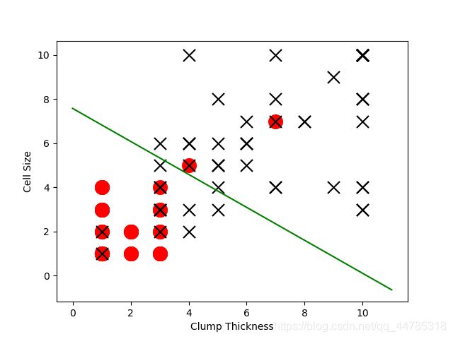
test_negative = test.loc[test['Type'] == 0][['Clump Thickness','Cell Size']]
test_positive = test.loc[test['Type'] == 1][['Clump Thickness','Cell Size']]
#以最终更新的参数作图
plt.scatter(test_negative['Clump Thickness'],test_negative['Cell Size'],marker='o',s=200,c='red')
plt.scatter(test_positive['Clump Thickness'],test_positive['Cell Size'],marker='x',s=150,c='black')
plt.xlabel('Clump Thickness')
plt.ylabel("Cell Size")
#取0-11个数当x值
lx = np.arange(0,12)
#计算12个X对应的y值
#这里要强调一下,我们以0.5作为分界面,所有计算方式如下,0.5-b-wx
ly = (0.5 - sess.run(b) - lx * sess.run(W)[0][0]) / sess.run(W)[0][1]
print(sess.run(b))
print(sess.run(W))
plt.plot(lx,ly,color = 'green')
plt.show()
结果:
200 [[0.01551242 0.12061065]] [-0.09584526]
400 [[0.05568662 0.08001342]] [-0.08955325]
600 [[0.05773812 0.07763022]] [-0.08739269]
800 [[0.05785108 0.07744841]] [-0.08697367]
1000 [[0.05785864 0.07742859]] [-0.08690023]
1200 [[0.05785936 0.07742577]] [-0.08688771]
1400 [[0.05785941 0.07742535]] [-0.08688553]
1600 [[0.05785941 0.07742535]] [-0.08688553]
1800 [[0.05785941 0.07742535]] [-0.08688553]
2000 [[0.05785941 0.07742535]] [-0.08688553]
[-0.08688553]
[[0.05785941 0.07742535]]