DGM: A deep learning algorithm for solving partial differential equations
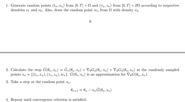
论文信息
题目:
DGM: A deep learning algorithm for solving partial differential equations
作者及单位:
Justin Sirignano∗ and Konstantinos Spiliopoulos
期刊、会议:
时间:18
论文地址:论文链接
代码:
基础
论文动机
- High-dimensional partial differential equations (PDEs) are used in physics, engineering, and finance. Their numerical solution has been a longstanding challenge
- This quickly becomes computationally intractable when the dimension d becomes even moderately large. We propose to solve high-dimensional PDEs
using a meshfree deep learning algorithm. - The method is similar in spirit to the Galerkin method, but with several key changes
using ideas from machine learning. - The Galerkin method is a widely-used computational method which seeks a reduced-form solution to a PDE as a linear combinationof basis functions.
- DGM is a natural
merger of Galerkin methods and machine learning
问题背景
本文方法
Approximation Power of Neural Networks for PDEs
∂ t u ( t , x ) + L u ( t , x ) = 0 , ( t , x ) ∈ [ 0 , T ] × Ω u ( 0 , x ) = u 0 ( x ) , x ∈ Ω u ( t , x ) = g ( t , x ) , x ∈ [ 0 , T ] × ∂ Ω \begin{array}{ll} \partial_{t} u(t, x)+\mathcal{L} u(t, x)=0, & (t, x) \in[0, T] \times \Omega \\ u(0, x)=u_{0}(x), & x \in \Omega \\ u(t, x)=g(t, x), & x \in[0, T] \times \partial \Omega \end{array} ∂tu(t,x)+Lu(t,x)=0,u(0,x)=u0(x),u(t,x)=g(t,x),(t,x)∈[0,T]×Ωx∈Ωx∈[0,T]×∂Ω
The error function:
J ( f ) = ∥ ∂ t f + L f ∥ 2 , [ 0 , T ] × Ω 2 + ∥ f − g ∥ 2 , [ 0 , T ] × ∂ Ω 2 + ∥ f ( 0 , ⋅ ) − u 0 ∥ 2 , Ω 2 J(f)=\left\|\partial_{t} f+\mathcal{L} f\right\|_{2,[0, T] \times \Omega}^{2}+\|f-g\|_{2,[0, T] \times \partial \Omega}^{2}+\left\|f(0, \cdot)-u_{0}\right\|_{2, \Omega}^{2} J(f)=∥∂tf+Lf∥2,[0,T]×Ω2+∥f−g∥2,[0,T]×∂Ω2+∥f(0,⋅)−u0∥2,Ω2
This paper explores several new innovations:
- First, we focus on
high-dimensional PDEs and apply deep learning advances of the past decade to this problem. - Secondly, to avoid ever forming a mesh, we
sample a sequence of random spatial points. - Thirdly, the algorithm incorporates
a new computational scheme for the efficient computationof neural network gradients arising from thesecond derivativesof high-dimensional PDEs.
DGM

A Monte Carlo Method for Fast Computation of Second Derivatives
包含二阶导数项得在计算高维时计算代价可能很昂贵,计算二阶导数代价(以4.2网络结构为例)是 O ( d 2 × N ) \mathcal{O}\left(d^{2} \times N\right) O(d2×N),其中d为x的空间维度,N为batch size,相比之下,一阶导数为 O ( d × N ) \mathcal{O}(d \times N) O(d×N),而且含有二阶导数项计算花费甚至更多,因为在梯度算法优化还会求一阶导数(相当于三阶导数),考虑到这些情况,二阶导数采用Monte Carlo方法.
假设 L f ( t , x , ; θ ) \mathcal{L} f(t, x, ; \theta) Lf(t,x,;θ)中二阶导数形式为 1 2 ∑ i , j = 1 d ρ i , j σ i ( x ) σ j ( x ) ∂ 2 f ∂ x i x j ( t , x ; θ ) \frac{1}{2} \sum_{i, j=1}^{d} \rho_{i, j} \sigma_{i}(x) \sigma_{j}(x) \frac{\partial^{2} f}{\partial x_{i} x_{j}}(t, x ; \theta) 21∑i,j=1dρi,jσi(x)σj(x)∂xixj∂2f(t,x;θ),假设 [ ρ i , j ] i , j = 1 d \left[\rho_{i, j}\right]_{i, j=1}^{d} [ρi,j]i,j=1d是正定矩阵同时定义 σ ( x ) = ( σ 1 ( x ) , … , σ d ( x ) ) \sigma(x)=\left(\sigma_{1}(x), \ldots, \sigma_{d}(x)\right) σ(x)=(σ1(x),…,σd(x)).这里 σ \sigma σ代表什么?例如,在考虑随机微分方程的期望的时候会产生偏微分方程时代表扩散系数(diffusion coefficient)。二阶项考虑如下计算:
∑ i , j = 1 d ρ i , j σ i ( x ) σ j ( x ) ∂ 2 f ∂ x i x j ( t , x ; θ ) = lim Δ → 0 E [ ∑ i = 1 d ∂ f ∂ x i ( t , x + σ ( x ) W Δ ; θ ) − ∂ f ∂ x i ( t , x ; θ ) Δ σ i ( x ) W Δ i ] \sum_{i, j=1}^{d} \rho_{i, j} \sigma_{i}(x) \sigma_{j}(x) \frac{\partial^{2} f}{\partial x_{i} x_{j}}(t, x ; \theta)=\lim _{\Delta \rightarrow 0} \mathbb{E}\left[\sum_{i=1}^{d} \frac{\frac{\partial f}{\partial x_{i}}\left(t, x+\sigma(x) W_{\Delta} ; \theta\right)-\frac{\partial f}{\partial x_{i}}(t, x ; \theta)}{\Delta} \sigma_{i}(x) W_{\Delta}^{i}\right] i,j=1∑dρi,jσi(x)σj(x)∂xixj∂2f(t,x;θ)=Δ→0limE[i=1∑dΔ∂xi∂f(t,x+σ(x)WΔ;θ)−∂xi∂f(t,x;θ)σi(x)WΔi]
其中, W t ∈ R d W_{t} \in \mathbb{R}^{d} Wt∈Rd 是一个布朗运动(Brownian motion), Δ ∈ R + \Delta \in \mathbb{R}_{+} Δ∈R+是步长,二阶替代后收敛速率为 O ( Δ ) \mathcal{O}(\sqrt{\Delta}) O(Δ)
从而一阶导数算子:
L 1 f ( t n , x n ; θ n ) : = L f ( t n , x n ; θ n ) − 1 2 ∑ i , j = 1 d ρ i , j σ i ( x n ) σ j ( x n ) ∂ 2 f ∂ x i x j ( t n , x n ; θ ) \mathcal{L}_{1} f\left(t_{n}, x_{n} ; \theta_{n}\right):=\mathcal{L} f\left(t_{n}, x_{n} ; \theta_{n}\right)-\frac{1}{2} \sum_{i, j=1}^{d} \rho_{i, j} \sigma_{i}\left(x_{n}\right) \sigma_{j}\left(x_{n}\right) \frac{\partial^{2} f}{\partial x_{i} x_{j}}\left(t_{n}, x_{n} ; \theta\right) L1f(tn,xn;θn):=Lf(tn,xn;θn)−21i,j=1∑dρi,jσi(xn)σj(xn)∂xixj∂2f(tn,xn;θ)
前面DGM定义的损失
G 1 ( θ n , s n ) : = ( ∂ f ∂ t ( t n , x n ; θ n ) + L f ( t n , x n ; θ n ) ) 2 G 2 ( θ n , s n ) : = ( f ( τ n , z n ; θ n ) − g ( τ n , z n ) ) 2 G 3 ( θ n , s n ) : = ( f ( 0 , w n ; θ n ) − u 0 ( w n ) ) 2 G ( θ n , s n ) : = G 1 ( θ n , s n ) + G 2 ( θ n , s n ) + G 3 ( θ n , s n ) \begin{array}{l} G_{1}\left(\theta_{n}, s_{n}\right):=\left(\frac{\partial f}{\partial t}\left(t_{n}, x_{n} ; \theta_{n}\right)+\mathcal{L} f\left(t_{n}, x_{n} ; \theta_{n}\right)\right)^{2} \\ G_{2}\left(\theta_{n}, s_{n}\right):=\left(f\left(\tau_{n}, z_{n} ; \theta_{n}\right)-g\left(\tau_{n}, z_{n}\right)\right)^{2} \\ G_{3}\left(\theta_{n}, s_{n}\right):=\left(f\left(0, w_{n} ; \theta_{n}\right)-u_{0}\left(w_{n}\right)\right)^{2} \\ G\left(\theta_{n}, s_{n}\right):=G_{1}\left(\theta_{n}, s_{n}\right)+G_{2}\left(\theta_{n}, s_{n}\right)+G_{3}\left(\theta_{n}, s_{n}\right) \end{array} G1(θn,sn):=(∂t∂f(tn,xn;θn)+Lf(tn,xn;θn))2G2(θn,sn):=(f(τn,zn;θn)−g(τn,zn))2G3(θn,sn):=(f(0,wn;θn)−u0(wn))2G(θn,sn):=G1(θn,sn)+G2(θn,sn)+G3(θn,sn)
DGM算法中用到梯度 ∇ θ G 1 ( θ n , s n ) \nabla_{\theta} G_{1}\left(\theta_{n}, s_{n}\right) ∇θG1(θn,sn)近视为 G ~ 1 \tilde{G}_{1} G~1估计,有固定项 Δ > 0 \Delta>0 Δ>0
G ~ 1 ( θ n , s n ) : = 2 ( ∂ f ∂ t ( t n , x n ; θ n ) + L 1 f ( t n , x n ; θ n ) + 1 2 ∑ i = 1 d ∂ f ∂ x i ( t , x n + σ ( x n ) W Δ ; θ ) − ∂ f ∂ x i ( t , x n ; θ ) Δ σ i ( x n ) W Δ i ) × ∇ θ ( ∂ f ∂ t ( t n , x n ; θ n ) + L 1 f ( t n , x n ; θ n ) + 1 2 ∑ i = 1 d ∂ f ∂ x i ( t , x n + σ ( x n ) W ~ Δ ; θ ) − ∂ f ∂ x i ( t , x n ; θ ) Δ σ i ( x n ) W ~ Δ i ) \begin{aligned} \tilde{G}_{1}\left(\theta_{n}, s_{n}\right):=& 2\left(\frac{\partial f}{\partial t}\left(t_{n}, x_{n} ; \theta_{n}\right)+\mathcal{L}_{1} f\left(t_{n}, x_{n} ; \theta_{n}\right)+\frac{1}{2} \sum_{i=1}^{d} \frac{\frac{\partial f}{\partial x_{i}}\left(t, x_{n}+\sigma\left(x_{n}\right) W_{\Delta} ; \theta\right)-\frac{\partial f}{\partial x_{i}}\left(t, x_{n} ; \theta\right)}{\Delta} \sigma_{i}\left(x_{n}\right) W_{\Delta}^{i}\right) \\ \times & \nabla_{\theta}\left(\frac{\partial f}{\partial t}\left(t_{n}, x_{n} ; \theta_{n}\right)+\mathcal{L}_{1} f\left(t_{n}, x_{n} ; \theta_{n}\right)+\frac{1}{2} \sum_{i=1}^{d} \frac{\frac{\partial f}{\partial x_{i}}\left(t, x_{n}+\sigma\left(x_{n}\right) \tilde{W}_{\Delta} ; \theta\right)-\frac{\partial f}{\partial x_{i}}\left(t, x_{n} ; \theta\right)}{\Delta} \sigma_{i}\left(x_{n}\right) \tilde{W}_{\Delta}^{i}\right) \end{aligned} G~1(θn,sn):=×2(∂t∂f(tn,xn;θn)+L1f(tn,xn;θn)+21i=1∑dΔ∂xi∂f(t,xn+σ(xn)WΔ;θ)−∂xi∂f(t,xn;θ)σi(xn)WΔi)∇θ⎝⎛∂t∂f(tn,xn;θn)+L1f(tn,xn;θn)+21i=1∑dΔ∂xi∂f(t,xn+σ(xn)W~Δ;θ)−∂xi∂f(t,xn;θ)σi(xn)W~Δi⎠⎞
其中, W Δ W_{\Delta} WΔ是d维正态随机变量,且满足 E [ W Δ ] = 0 \mathbb{E}\left[W_{\Delta}\right]=0 E[WΔ]=0以及 Cov [ ( W Δ ) i , ( W Δ ) i ] = ρ i , i Δ \operatorname{Cov}\left[\left(W_{\Delta}\right)_{i},\left(W_{\Delta}\right)_{i}\right]=\rho_{i, i} \Delta Cov[(WΔ)i,(WΔ)i]=ρi,iΔ. W ~ Δ \tilde{W}_{\Delta} W~Δ有和 W Δ W_{\Delta} WΔ一样的分布. G ~ 1 ( θ n , s n ) \tilde{G}_{1}\left(\theta_{n}, s_{n}\right) G~1(θn,sn)是,KaTeX parse error: Expected '\right', got 'EOF' at end of input: …eft(\theta_{n}是\nabla_{\theta} G_{1}\left(\theta_{n}, s_{n}\right)KaTeX parse error: Expected 'EOF', got '\right' at position 23: …Carlo的估计, s_{n}\̲r̲i̲g̲h̲t̲)有 O ( Δ ) \mathcal{O}(\sqrt{\Delta}) O(Δ)偏差. 这种误差可以根据下面的估计方法改进
G ~ 1 ( θ n , s n ) : = G ~ 1 , a ( θ n , s n ) + G ~ 1 , b ( θ n , s n ) \tilde{G}_{1}\left(\theta_{n}, s_{n}\right) \quad:=\quad \tilde{G}_{1, a}\left(\theta_{n}, s_{n}\right)+\tilde{G}_{1, b}\left(\theta_{n}, s_{n}\right) G~1(θn,sn):=G~1,a(θn,sn)+G~1,b(θn,sn)
G ~ 1 , a ( θ n , s n ) : = ( ∂ f ∂ t ( t n , x n ; θ n ) + L 1 f ( t n , x n ; θ n ) + 1 2 ∑ i = 1 a ∂ J ∂ x i ( t , x n + σ ( x n ) W Δ ; θ ) − σ j ∂ x i ( t , x n ; θ ) Δ σ i ( x n ) W Δ i ) × ∇ θ ( ∂ f ∂ t ( t n , x n ; θ n ) + L 1 f ( t n , x n ; θ n ) + 1 2 ∑ i = 1 d ∂ f ∂ x i ( t , x n + σ ( x n ) W ~ Δ ; θ ) − ∂ f ∂ x i ( t , x n ; θ ) Δ σ i ( x n ) W ~ Δ i ) \begin{aligned} \tilde{G}_{1, a}\left(\theta_{n}, s_{n}\right): &=\left(\frac{\partial f}{\partial t}\left(t_{n}, x_{n} ; \theta_{n}\right)+\mathcal{L}_{1} f\left(t_{n}, x_{n} ; \theta_{n}\right)+\frac{1}{2} \sum_{i=1}^{a} \frac{\frac{\partial J}{\partial x_{i}}\left(t, x_{n}+\sigma\left(x_{n}\right) W_{\Delta} ; \theta\right)-\frac{\sigma_{j}}{\partial x_{i}}\left(t, x_{n} ; \theta\right)}{\Delta} \sigma_{i}\left(x_{n}\right) W_{\Delta}^{i}\right) \\ & \times \nabla_{\theta}\left(\frac{\partial f}{\partial t}\left(t_{n}, x_{n} ; \theta_{n}\right)+\mathcal{L}_{1} f\left(t_{n}, x_{n} ; \theta_{n}\right)+\frac{1}{2} \sum_{i=1}^{d} \frac{\frac{\partial f}{\partial x_{i}}\left(t, x_{n}+\sigma\left(x_{n}\right) \tilde{W}_{\Delta} ; \theta\right)-\frac{\partial f}{\partial x_{i}}\left(t, x_{n} ; \theta\right)}{\Delta} \sigma_{i}\left(x_{n}\right) \tilde{W}_{\Delta}^{i}\right) \end{aligned} G~1,a(θn,sn):=(∂t∂f(tn,xn;θn)+L1f(tn,xn;θn)+21i=1∑aΔ∂xi∂J(t,xn+σ(xn)WΔ;θ)−∂xiσj(t,xn;θ)σi(xn)WΔi)×∇θ⎝⎛∂t∂f(tn,xn;θn)+L1f(tn,xn;θn)+21i=1∑dΔ∂xi∂f(t,xn+σ(xn)W~Δ;θ)−∂xi∂f(t,xn;θ)σi(xn)W~Δi⎠⎞
KaTeX parse error: Undefined control sequence: \su at position 623: …t)-\frac{1}{2} \̲s̲u̲ ̲ ̲ ̲ ̲ ̲ ̲ ̲ ̲ ̲ ̲ ̲ ̲ ̲ ̲ ̲ ̲ ̲ ̲ ̲ ̲ ̲ ̲ ̲ ̲ ̲ ̲ ̲ ̲ ̲ ̲ ̲ ̲ ̲ ̲ ̲ ̲ ̲ ̲ ̲ ̲ ̲ ̲m_{i=1}^{d} \fr…
上面的估计方法有 O ( Δ ) \mathcal{O}(\Delta) O(Δ)的偏差
- The computational cost for calculating second derivatives
The modified algorithm here is computationally less expensive than the original algorithm
Relevant literature
- Recently, Raissi [41, 42] develop physics informed deep learning models. They estimate deep neural network models which
merge data observations with PDE models. This allows for the estimation of physical models from limited data by leveraging a priori knowledge that the physical dynamics should obey a class of PDEs. Their approach solves PDEsin one and two spatial dimensions using deep neural networks.
[33] developed an algorithm for the solution of a discrete-time version of a class of free boundary PDEs. - Their algorithm, commonly called the Longstaff-Schwartz method", uses dynamic programming and approximates the solution
using a separate function approximator at each discrete time(typically a linear combination of basis functions).Our algorithm directly solves the PDE, and uses a single function approximator for all space and all time.
数值实验
The Free Boundary PDE
Free boundary PDE and will satisfy
0 = ∂ u ∂ t ( t , x ) + μ ( x ) ⋅ ∂ u ∂ x ( t , x ) + 1 2 ∑ i , j = 1 d ρ i , j σ ( x i ) σ ( x j ) ∂ 2 u ∂ x i ∂ x j ( t , x ) − r u ( t , x ) , ∀ { ( t , x ) : u ( t , x ) > g ( x ) } u ( t , x ) ≥ g ( x ) , ∀ ( t , x ) u ( t , x ) ∈ C 1 ( R + × R d ) , ∀ { ( t , x ) : u ( t , x ) = g ( x ) } u ( T , x ) = g ( x ) , ∀ x \begin{aligned} 0 &=\frac{\partial u}{\partial t}(t, x)+\mu(x) \cdot \frac{\partial u}{\partial x}(t, x)+\frac{1}{2} \sum_{i, j=1}^{d} \rho_{i, j} \sigma\left(x_{i}\right) \sigma\left(x_{j}\right) \frac{\partial^{2} u}{\partial x_{i} \partial x_{j}}(t, x)-r u(t, x), \quad \forall\{(t, x): u(t, x)>g(x)\} \\ u(t, x) & \geq g(x), \quad \forall(t, x) \\ u(t, x) & \in C^{1}\left(\mathbb{R}_{+} \times \mathbb{R}^{d}\right), \quad \forall\{(t, x): u(t, x)=g(x)\} \\ u(T, x) &=g(x), \quad \forall x \end{aligned} 0u(t,x)u(t,x)u(T,x)=∂t∂u(t,x)+μ(x)⋅∂x∂u(t,x)+21i,j=1∑dρi,jσ(xi)σ(xj)∂xi∂xj∂2u(t,x)−ru(t,x),∀{(t,x):u(t,x)>g(x)}≥g(x),∀(t,x)∈C1(R+×Rd),∀{(t,x):u(t,x)=g(x)}=g(x),∀x
Implementation details for the algorithm
在训练过程使用了多块GPU,为了加速训练,使用了异步随机梯度下降(asynchronous stochastic gradient descent),这是机器学习模型中应用广泛的并行训练方法. Figure 1 displays the computational setup

A High-dimensional Free Boundary PDE with a Semi-Analytic Solution
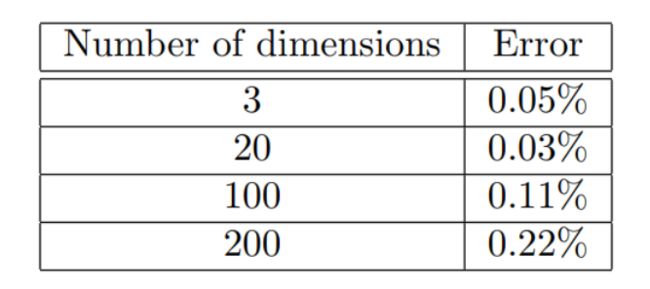
The accuracy of our deep learning algorithm is evaluated in up to 200 dimensions
We present in Figure 2 contour plots of the absolute error and percent error across time and space for the American option PDE in 20 dimensions.
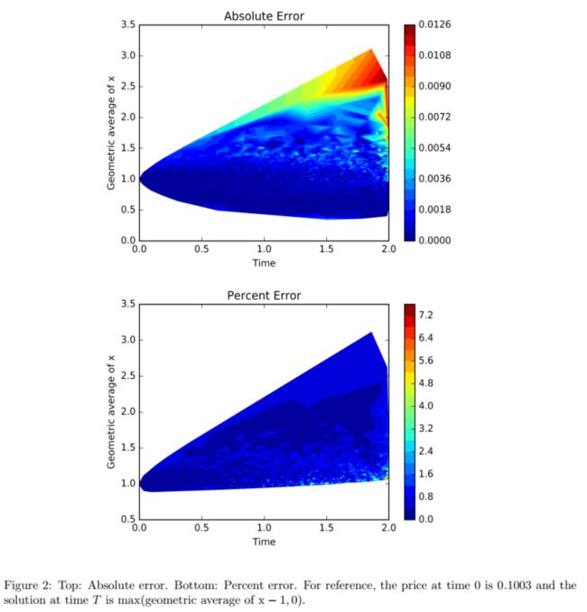
Figure 2 reports both the absolute error and the percent error. The percent error ∣ f ( t , x ; θ ) − u ( t , x ) ∣ ∣ u ( t , x ) ∣ × 100 % \frac{|f(t, x ; \theta)-u(t, x)|}{|u(t, x)|} \times 100 \% ∣u(t,x)∣∣f(t,x;θ)−u(t,x)∣×100% is reported for points where ∣ u ( t , x ) ∣ > 0.05 |u(t, x)|>0.05 ∣u(t,x)∣>0.05. The absolute error becomes relatively large in a few areas;however, the solution u(t; x) also grows large in these areas and therefore the percent error remains small
Burgers’ equation
∂ u ∂ t ( t , x ; p ) = L p u ( t , x ; p ) , ( t , x ) ∈ [ 0 , T ] × Ω u ( t , x ; p ) = g p ( x ) , ( t , x ) ∈ [ 0 , T ] × ∂ Ω u ( t = 0 , x ; p ) = h p ( x ) , x ∈ Ω \begin{aligned} \frac{\partial u}{\partial t}(t, x ; p) &=\mathcal{L}_{p} u(t, x ; p), \quad(t, x) \in[0, T] \times \Omega \\ u(t, x ; p) &=g_{p}(x), \quad(t, x) \in[0, T] \times \partial \Omega \\ u(t=0, x ; p) &=h_{p}(x), \quad x \in \Omega \end{aligned} ∂t∂u(t,x;p)u(t,x;p)u(t=0,x;p)=Lpu(t,x;p),(t,x)∈[0,T]×Ω=gp(x),(t,x)∈[0,T]×∂Ω=hp(x),x∈Ω
A traditional approach would be to discretize the P-space and re-solve the PDE many times for many different points p. However, the total number of grid points (and therefore the number of PDEs that must be solved) grows exponentially with the number of dimensions, and P is typically high-dimensional.
We use DGM to solve the PDE as follows:

We consider the following burge equation:
∂ u ∂ t = ν ∂ 2 u ∂ x 2 − α u ∂ u ∂ x , ( t , x ) ∈ [ 0 , 1 ] × [ 0 , 1 ] \frac{\partial u}{\partial t}=\nu \frac{\partial^{2} u}{\partial x^{2}}-\alpha u \frac{\partial u}{\partial x}, \quad(t, x) \in[0,1] \times[0,1] ∂t∂u=ν∂x2∂2u−αu∂x∂u,(t,x)∈[0,1]×[0,1]
u ( t , x = 0 ) = a u(t, x=0)=a u(t,x=0)=a
u ( t , x = 1 ) = b u(t, x=1)=b u(t,x=1)=b
u ( t = 0 , x ) = g ( x ) , x ∈ [ 0 , 1 ] u(t=0, x)=g(x), \quad x \in[0,1] u(t=0,x)=g(x),x∈[0,1]
The problem setup space is P = ( ν , α , a , b ) ∈ R 4 \mathcal{P}=(\nu, \alpha, a, b) \in \mathbb{R}^{4} P=(ν,α,a,b)∈R4, the entire space ( t , x , ν , α , a , b ) ∈ [ 0 , 1 ] × [ 0 , 1 ] × [ 1 0 − 2 , 1 0 − 1 ] × [ 1 0 − 2 , 1 ] × [ − 1 , 1 ] × [ − 1 , 1 ] (t, x, \nu, \alpha, a, b) \in[0,1] \times[0,1] \times[10^{-2}, 10^{-1}] \times [10^{-2}, 1] \times[-1,1] \times[-1,1] (t,x,ν,α,a,b)∈[0,1]×[0,1]×[10−2,10−1]×[10−2,1]×[−1,1]×[−1,1]
Figure 5 compares the deep learning solution with the exact solution for
several different problem setups p

Figure 5 compares the deep learning solution with the exact solution for several different problem setups p. The solutions are very close; in several cases, the two solutions are visibly indistinguishable. The deep learning algorithm is able to accurately capture the shock layers and boundary layers.
Neural Network Approximation Theorem for PDEs
Figure 6 presents the accuracy of the deep learning algorithm for different times t and different choices of ν.
总结:
- We prove that the neural network converges to the solution of the partial differential equation as the number of hidden units increases.
- Stability analysis of deep learning and machine learning algorithms for solving PDEs is also an important question. It would certainly be interesting to study machine learning algorithms that use a more direct variational formulation of the involved PDEs. We
leave these questions for future work