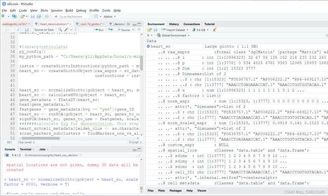
Heart_deconvolution giotto解卷积

---

title: “Heart_deconvolution”
#https://github.com/rdong08/spatialDWLS_dataset
output: html_document

#https://github.com/rdong08/spatialDWLS_dataset/blob/main/codes/Heart_ST_tutorial_spatialDWLS.Rmd

##Import library

```{r}

library(Giotto)
library(ggplot2)
library(scatterpie)
library(data.table)
#getwd() path="G:/silicosis/sicosis/gitto/heart_visu_deconv/" setwd(path) ##Here is an example for tutorial by using spatial transcriptomic data of Sample 10, W6 in Asp et al. ##Identification of marker gene expression in single cell #{r}
#sc_meta<-read.table("…/datasets/heart_development_ST/sc_meta.txt",header = F,row.names = 1)
#sc_data<-read.table("…/datasets/heart_development_ST/all_cells_count_matrix_filtered.tsv",header = T,row.names = 1)

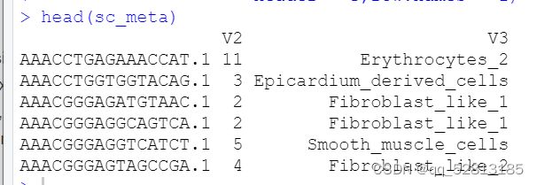
sc_meta=read.table(“G:/silicosis/sicosis/gitto/heart_visu_deconv/sc_meta.txt”,
header =FALSE,row.names = 1)
head(sc_meta)

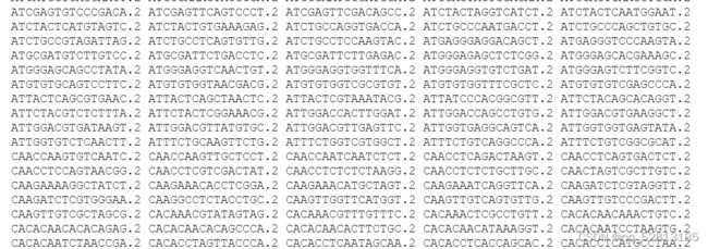
sc_data<-read.table(“G:/silicosis/sicosis/gitto/heart_visu_deconv/all_cells_count_matrix_filtered.tsv/all_cells_count_matrix_filtered.tsv”,
header = T,row.names = 1)
head(sc_data)

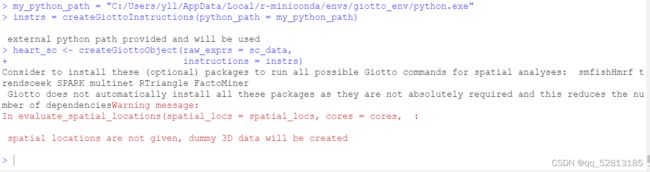
my_python_path = “python path”
instrs = createGiottoInstructions(python_path = my_python_path)
heart_sc <- createGiottoObject(raw_exprs = sc_data,
instructions = instrs)

heart_sc <- normalizeGiotto(gobject = heart_sc, scalefactor = 6000, verbose = T)

heart_sc <- calculateHVG(gobject = heart_sc)

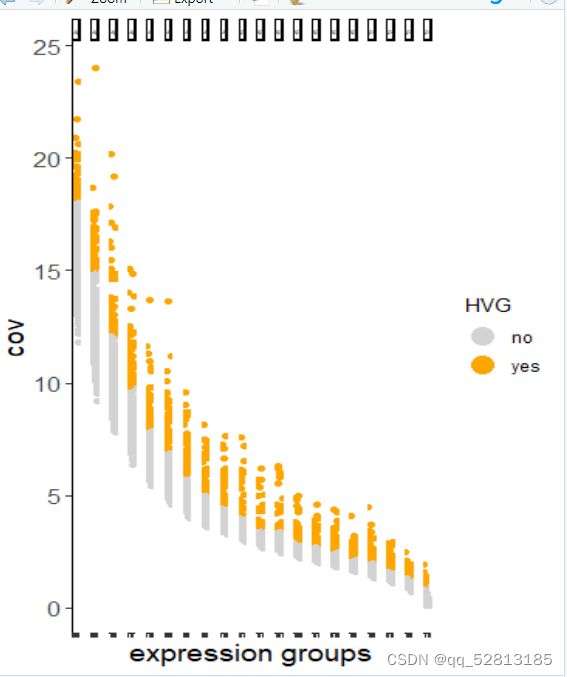
gene_metadata = fDataDT(heart_sc)
featgenes = gene_metadata[hvg == ‘yes’]$gene_ID

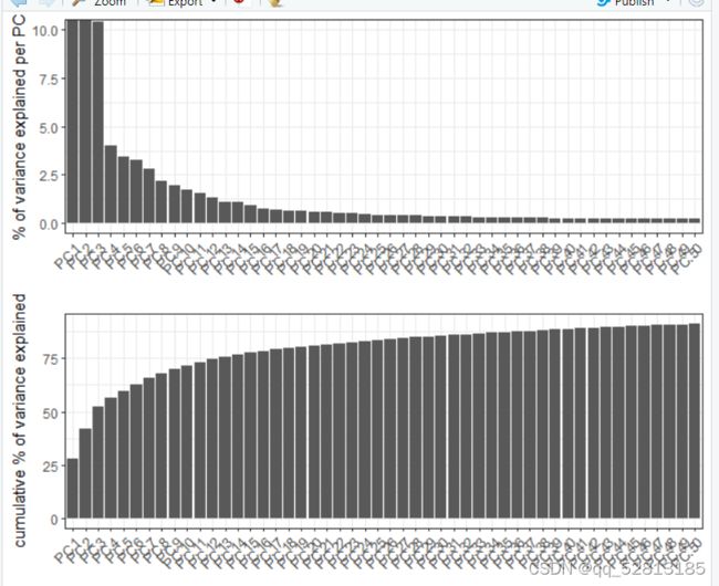
heart_sc <- runPCA(gobject = heart_sc, genes_to_use = featgenes, scale_unit = F)
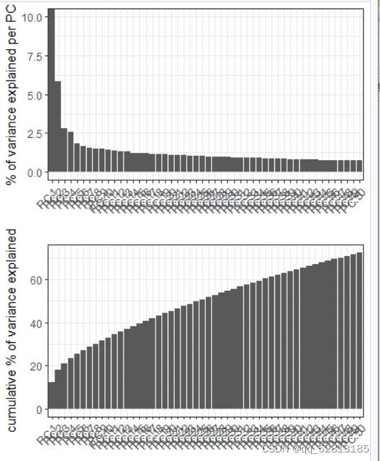
signPCA(heart_sc, genes_to_use = featgenes, scale_unit = F)

#######calculate Sig for deconvolution, This step use DEG function implemented in Giotto

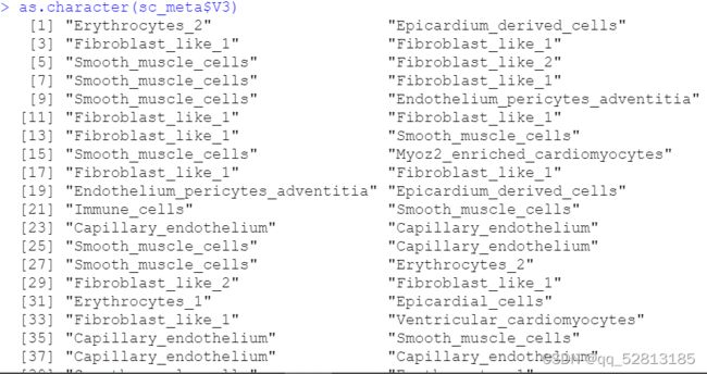
heart_sc@cell_metadata$leiden_clus <- as.character(sc_meta$V3)

scran_markers_subclusters = findMarkers_one_vs_all(gobject = heart_sc,
method = ‘scran’,
expression_values = ‘normalized’,
cluster_column = ‘leiden_clus’)

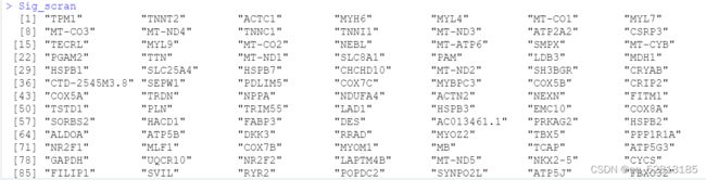
Sig_scran <- unique(scran_markers_subclusters$genes[which(scra{n}_{m}arker{s}_{s}ubclusters$ranking <= 100)])

########Calculate median expression value of signature genes in each cell type

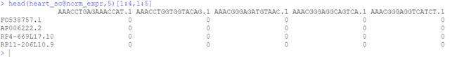
norm_exp<-2^(heart_sc@norm_expr)-1

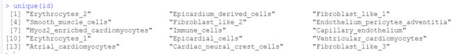
id<-heart_sc@cell_metadata$leiden_clus
ExprSubset<-norm_exp[Sig_scran,]

Sig_exp<-NULL

for (i in unique(id)){
Sig_exp<-cbind(Sig_exp,(apply(ExprSubset,1,function(y) mean(y[which(id==i)]))))
}
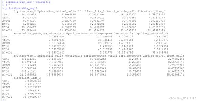
colnames(Sig_exp)<-unique(id)
#```

##Spatial transcriptomic data analysis
#```{r}
##The heart spatial transcriptomic data is from Asp et al “A Spatiotemporal Organ-Wide Gene Expression and Cell Atlas of the Developing Human Heart”.
spatial_loc<-read.table(file="…/datasets/heart_development_ST/sample10_w6_loc.txt",header = F)

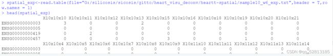
spatial_exp<-read.table(file="…/datasets/heart_development_ST/sample10_w6_exp.txt",header = T,row.names = 1)

##Transform ensemble gene to official gene name
ens2gene<-read.table(file="…/datasets/heart_development_ST/ens2symbol.txt",row.names = 1)

inter_ens<-intersect(rownames(spatial_exp),rownames(ens2gene))

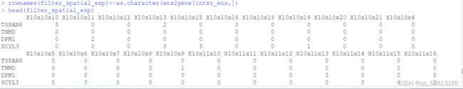
filter_spatial_exp<-spatial_exp[inter_ens,]
rownames(filter_spatial_exp)<-as.character(ens2gene[inter_ens,])

##Generate Giotto objects and cluster spots
heart_w6_sample10_st <- createGiottoObject(raw_exprs = filter_spatial_exp,spatial_locs = spatial_loc,
instructions = instrs)
heart_w6_sample10_st <- filterGiotto(gobject = heart_w6_sample10_st,
expression_threshold = 1,
gene_det_in_min_cells = 10,
min_det_genes_per_cell = 200,
expression_values = c(‘raw’),
verbose = T)

heart_w6_sample10_st <- normalizeGiotto(gobject = heart_w6_sample10_st)
heart_w6_sample10_st <- calculateHVG(gobject = heart_w6_sample10_st)
gene_metadata = fDataDT(heart_w6_sample10_st)

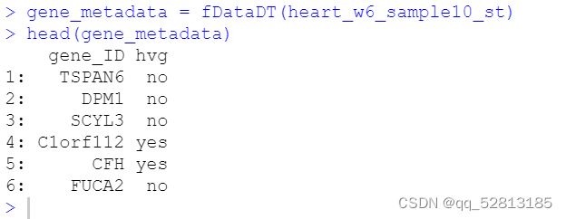
featgenes = gene_metadata[hvg == ‘yes’]$gene_ID
heart_w6_sample10_st <- runPCA(gobject = heart_w6_sample10_st, genes_to_use = featgenes, scale_unit = F)
signPCA(heart_w6_sample10_st, genes_to_use = featgenes, scale_unit = F)

heart_w6_sample10_st <- createNearestNetwork(gobject = heart_w6_sample10_st, dimensions_to_use = 1:10, k = 10)
heart_w6_sample10_st <- doLeidenCluster(gobject = heart_w6_sample10_st, resolution = 0.4, n_iterations = 1000)
##Deconvolution based on signature gene expression and Giotto object
heart_w6_sample10_st <- runDWLSDeconv(gobject = heart_w6_sample10_st, sign_matrix = Sig_exp)
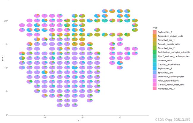
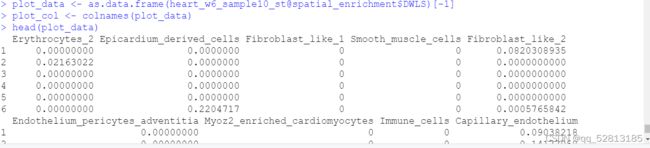
##The result for deconvolution is stored in heart_w6_sample10_st@spatial_enrichment$DWLS.Thefollowingcodesarevisualizationdeconvolutionresultsusingpieplotplo{t}_{d}ata<-as.data.frame(hear{t}_w{6}_{s}ample10_{s}t@spatia{l}_{e}nrichment$DWLS)[-1]
plot_col <- colnames(plot_data)

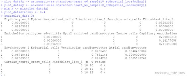
plot_data$x<-as.numeric(as.character(hear{t}_w{6}_{s}ample10_{s}t@spatia{l}_{l}ocs$sdimx))
plot_data$y<-as.numeric(as.character(hear{t}_w{6}_{s}ample10_{s}t@spatia{l}_{l}ocs$sdimy))
min_x <- min(plot_data$x)plo{t}_{d}ata$radius <- 0.4

df <- data.frame()
p <- ggplot(df) + geom_point() + xlim(min(plot_data$x)-1,max(plo{t}_{d}ata$x)+1) + ylim(min(plot_data$y)-1,max(plo{t}_{d}ata$y)+1)
p + geom_scatterpie(aes(x=x, y=y, r=radius), data=plot_data, cols=plot_col, color=NA, alpha=.8) +
geom_scatterpie_legend(plot_data$radius, x=1, y=1) + theme_classic()
#``