Python机器学习03——逻辑回归
本系列所有的代码和数据都可以从陈强老师的个人主页上下载:Python数据程序
参考书目:陈强.机器学习及Python应用. 北京:高等教育出版社, 2021.
本系列基本不讲数学原理,只从代码角度去让读者们利用最简洁的Python代码实现机器学习方法。
逻辑回归Python案例:
逻辑回归时用来做分类的,将数据经过非线性变化压缩到0~1之间就变为了概率,其逻辑分布和密度图为:

数据集介绍
采用泰坦尼克号数据集,响应变量为‘’是否生存‘’这个分类变量,首先读取数据和包,对数据进行一定的处理
import pandas as pd
import numpy as np
titanic = pd.read_csv('titanic.csv')
freq = titanic.Freq.to_numpy()
index = np.repeat(np.arange(32), freq)
index.shape
#构建索引 根据重复索引生存数据框
titanic = titanic.iloc[index,:]
titanic = titanic.drop('Freq', axis=1)
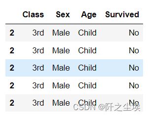
titanic.head()
数据最后长这个样子(前五行)
生产数据透视表
pd.crosstab(titanic.Class, titanic.Survived, normalize='index') 
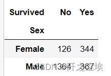
上面是每个属性的比例,生成数值的代码为
pd.crosstab(titanic.Sex, titanic.Survived)
sklearn库的逻辑回归
import matplotlib.pyplot as plt
from sklearn.linear_model import LogisticRegression
from sklearn.metrics import confusion_matrix
from sklearn.metrics import classification_report
from sklearn.metrics import cohen_kappa_score
首先取出X和y,对x生成虚拟变量
X = titanic.iloc[:,:-1]
y = titanic.iloc[:,-1]
X=pd.get_dummies(X,drop_first = True)
X 
划分训练集和测试集
from sklearn.model_selection import train_test_split
from sklearn.linear_model import LogisticRegression
X_train, X_test, y_train, y_test =  train_test_split(X,y,test_size=0.2, stratify=y, random_state=0)
进行拟合
model =  LogisticRegression(C=1e10)
model.fit(X_train, y_train)
考察模型的截距和回归系数
model.intercept_    #模型截距
model.coef_       #模型回归系数
测试集进行评价分类准确率
model.score(X_test, y_test) 预测所有种类的概率(只看前五个)
prob = model.predict_proba(X_test)
prob[:5]
预测所有种类(只看前五个)
pred = model.predict(X_test)
pred[:5]
画混淆矩阵
table = pd.crosstab(y_test, pred, rownames=['Actual'], colnames=['Predicted'])
table
计算混淆矩阵的指标
print(classification_report(y_test, pred, target_names=['Not Survived', 'Survived']))画ROC曲线
from scikitplot.metrics import plot_roc
plot_roc(y_test, prob)
x = np.linspace(0, 1, 100)
plt.plot(x, x, 'k--', linewidth=1)
plt.title('ROC Curve (Test Set)')
计算科恩Kappa指标
cohen_kappa_score(y_test, pred)
多分类的逻辑回归
上述泰坦尼克号采用的是二分类,多分类的逻辑回归也差不多,下面采用一个玻璃分类的数据集。
查看前五行
Glass = pd.read_csv('Glass.csv')
Glass.head()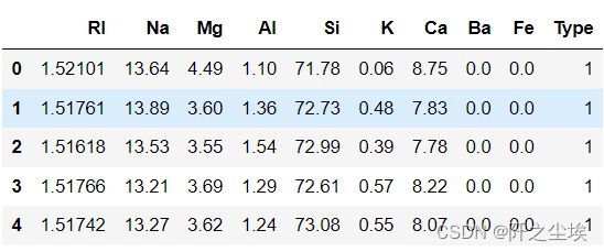
查看响应变量y的取值分布:
Glass.Type.value_counts()取出X,y,划分测试训练集,进行拟合
X = Glass.iloc[:,:-1]
y = Glass.iloc[:,-1]
#划分训练测试集
X_train, X_test, y_train, y_test =  train_test_split(X,y,test_size=0.3, stratify=y, random_state=0)
#生成逻辑回归类,multi_class='multinomial'表示多分类
model =  LogisticRegression(multi_class='multinomial', solver = 'newton-cg', C=1e10, max_iter=1e3)
model.fit(X_train, y_train)  #拟合
model.n_iter_  #查看迭代次数
model.intercept_  #查看截距
model.coef_    # 查看回归系数
model.score(X_test, y_test)   #查看测试集上的准确率
查看前三个预测的种类概率,六分类问题,所以一组是六个概率
prob = model.predict_proba(X_test)
prob[:3]
预测类别,查看前五个
pred = model.predict(X_test)
pred[:5] ![]()
画混淆矩阵
table = pd.crosstab(y_test, pred, rownames=['Actual'], colnames=['Predicted'])
table
画混淆矩阵热力图
import matplotlib.pyplot as plt
import seaborn as sns
sns.heatmap(table,cmap='Blues', annot=True)
plt.tight_layout() 
#计算混淆矩阵的各项指标
print(classification_report(y_test, pred))
#科恩Kappa指标
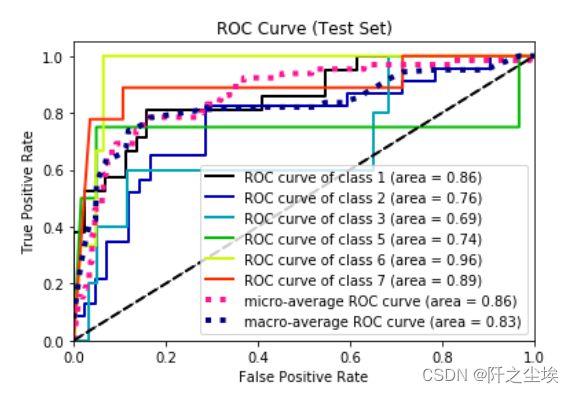
cohen_kappa_score(y_test, pred)画ROC曲线
from scikitplot.metrics import plot_roc
plot_roc(y_test, prob)
x = np.linspace(0, 1, 100)
plt.plot(x, x, 'k--', linewidth=1)
plt.title('ROC Curve (Test Set)')