365天深度学习训练营
LSTM-火灾温度预测
- 本文为365天深度学习训练营 中的学习记录博客
- 参考文章:第R2周:LSTM-火灾温度预测(训练营内部可读)
- 作者:K同学啊
任务说明
数据集中提供了火灾温度(Tem1)、一氧化碳浓度(CO 1)、烟雾浓度(Soot 1)随着时间变化数据,我们需要根据这些数据对未来某一时刻的火灾温度做出预测(本次任务仅供学习)
一、前期准备
import tensorflow as tf
gpus = tf.config.list_physical_devices("GPU")

if gpus:
    gpu0 = gpus[0] #如果有多个GPU,仅使用第0个GPU
    tf.config.experimental.set_memory_growth(gpu0, True) #设置GPU显存用量按需使用
    tf.config.set_visible_devices([gpu0],"GPU")
gpus
![]()
二、导入数据
import pandas     as pd
import numpy      as np

df_1 = pd.read_csv("G:/study/woodpine2.csv")
数据可视化
import matplotlib.pyplot as plt
import seaborn as sns

plt.rcParams['savefig.dpi'] = 500 #图片像素
plt.rcParams['figure.dpi']  = 500 #分辨率

fig, ax =plt.subplots(1,3,constrained_layout=True, figsize=(14, 3))

sns.lineplot(data=df_1["Tem1"], ax=ax[0])
sns.lineplot(data=df_1["CO 1"], ax=ax[1])
sns.lineplot(data=df_1["Soot 1"], ax=ax[2])
plt.show()

dataFrame = df_1.iloc[:,1:]
dataFrame

三、构建数据集
X=[]
y=[]
#取前8个时间段的Tem1,CO 1,Soot1为X,第九个时间段的Tem1为y
in_start = 0
for _, _ in df_1.iterrows():
in_end = in_start + width_X
out_end = in_end + width_y
if out_end < len(dataFrame):
X_ = np.array(dataFrame.iloc[in_start:in_end , ])
X_ = X_.reshape((len(X_)*3))
y_ = np.array(dataFrame.iloc[in_end :out_end, 0])
X.append(X_)
y.append(y_)
in_start += 1
X = np.array(X)
y = np.array(y)
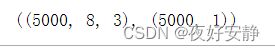
X.shape, y.shape

from sklearn.preprocessing import MinMaxScaler

#将数据归一化,范围是0到1
sc       = MinMaxScaler(feature_range=(0, 1))
X_scaled = sc.fit_transform(X)
X_scaled.shape
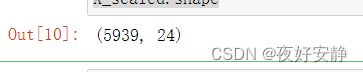
X_scaled = X_scaled.reshape(len(X_scaled),width_X,3)
X_scaled.shape

X_train = np.array(X_scaled[:5000]).astype('float64')
y_train = np.array(y[:5000]).astype('float64')

X_test  = np.array(X_scaled[5000:]).astype('float64')
y_test  = np.array(y[5000:]).astype('float64')
X_train.shape

四、构建模型
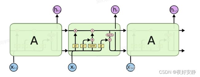
在上一周中,学习了RNN,并了解了RNN的一些优缺点,为了弥补RNN的一些不足,即长距离依赖,LSTM出现,LSTM(Long Short Time Memory networks)全称长短时记忆网络。
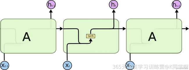
LSTM避免了长期依赖的问题。可以记住长期信息!LSTM内部有较为复杂的结构。能通过门控状态来选择调整传输的信息,记住需要长时间记忆的信息,忘记不重要的信息,其结构如下
from tensorflow.keras.models import Sequential
from tensorflow.keras.layers import Dense,LSTM,Bidirectional
from tensorflow.keras        import Input

# 多层 LSTM
model_lstm = Sequential()
model_lstm.add(LSTM(units=64, activation='relu', return_sequences=True,
               input_shape=(X_train.shape[1], 3)))
model_lstm.add(LSTM(units=64, activation='relu'))

model_lstm.add(Dense(width_y))
![]()
# 只观测loss数值,不观测准确率,所以删去metrics选项
model_lstm.compile(optimizer=tf.keras.optimizers.Adam(1e-3),
                   loss='mean_squared_error')  # 损失函数用均方误差
X_train.shape, y_train.shape
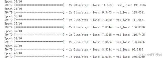
history_lstm = model_lstm.fit(X_train, y_train,
                         batch_size=64,
                         epochs=40,
                         validation_data=(X_test, y_test),
                         validation_freq=1)

# 支持中文
plt.rcParams['font.sans-serif'] = ['SimHei'] # 用来正常显示中文标签
plt.rcParams['axes.unicode_minus'] = False # 用来正常显示负号
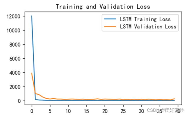
plt.figure(figsize=(5, 3),dpi=120)
plt.plot(history_lstm.history['loss'] , label='LSTM Training Loss')
plt.plot(history_lstm.history['val_loss'], label='LSTM Validation Loss')
plt.title('Training and Validation Loss')
plt.legend()
plt.show()
predicted_y_lstm = model_lstm.predict(X_test)                        # 测试集输入模型进行预测

y_test_one = [i[0] for i in y_test]
predicted_y_lstm_one = [i[0] for i in predicted_y_lstm]

plt.figure(figsize=(5, 3),dpi=120)
# 画出真实数据和预测数据的对比曲线
plt.plot(y_test_one[:1000], color='red', label='真实值')
plt.plot(predicted_y_lstm_one[:1000], color='blue', label='预测值')

plt.title('Title')
plt.xlabel('X')
plt.ylabel('Y')
plt.legend()
plt.show()

from sklearn import metrics
"""
RMSE :均方根误差 -----> 对均方误差开方
R2 :决定系数,可以简单理解为反映模型拟合优度的重要的统计量
"""
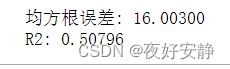
RMSE_lstm = metrics.mean_squared_error(predicted_y_lstm, y_test)**0.5
R2_lstm = metrics.r2_score(predicted_y_lstm, y_test)
print('均方根误差: %.5f' % RMSE_lstm)
print('R2: %.5f' % R2_lstm)