python数据分析与展示--Pandas库入门

一.Pandas库的引用

Pandas是python第三方库，通过了高性能易用的数据类型和分析工具;Pandas库包含了Series，DataFrame两个数据类型，基于这两个数据类型可以实现基本，运算，特征类，关联类操作

导入：

import pandas as pd

 小例：

import pandas as pd
d=pd.Series(range(20))
print(d)
'''
0      0
1      1
2      2
3      3
4      4
5      5
6      6
7      7
8      8
9      9
10    10
11    11
12    12
13    13
14    14
15    15
16    16
17    17
18    18
19    19
dtype: int64
'''

---

二.Pandas库的Serices类型

Series类型由一组数据及与之相关的数据索引组成

---

1.Series类型的创建

Series类型可以由如下类型创建：

·python列表：index与列表元素个数一致

·标量值：index的个数表示Series的个数

·python字典：键值对的‘键’是索引，index从字典中进行选择操作

·ndarray：通过ndarray创建索引和数据

·其他函数：range函数

---

 代码实例：

从列表创建：

import pandas as pd
d=pd.Series([2,6,4,8,3],index=['a','b','c','d','e'])
print(d)
'''
a    2
b    6
c    4
d    8
e    3
dtype: int64
'''

---

从标量值创建：

import pandas as pd
#从标量值创建不能省略indx
d=pd.Series(6,index=['a','b','c','d','e'])
print(d)
'''
a    6
b    6
c    6
d    6
e    6
dtype: int64
'''

---

从字典类型创建：

import pandas as pd
#从字典创建可以省略indx
d=pd.Series({'c':4,'d':7,'b':3,'a':2,'e':6},index=['a','b','c','d','e'])
print(d)
'''
a    2
b    3
c    4
d    7
e    6
dtype: int64
'''

---

从ndarray类型创建：

import pandas as pd
import numpy as np
#可以省略indx
d=pd.Series(np.arange(5),index=np.arange(9,4,-1))
print(d)
'''
9    0
8    1
7    2
6    3
5    4
dtype: int32
'''

---

2.Series类型的基本操作

（1）基于index和values的操作

import pandas as pd
a=pd.Series([9,8,7,6],['a','b','c','d'])
print('a:')
print(a)
print('a的数据:\n',a.values)     #.values获得数据
print('a的索引:\n',a.index)    #.index获得索引
print('索引取数据:\n',a[['d','c','a']])
'''
a:
a    9
b    8
c    7
d    6
dtype: int64
a的值:
 [9 8 7 6]
a的索引:
 Index(['a', 'b', 'c', 'd'], dtype='object')
 索引取数据:
 d    6
c    7
a    9
dtype: int64
'''

---

（2）Series类型类似ndarray类型的操作

·索引方法相同，采用[ ]

·NumPy中运算和操作可用于Series类型

·可以通过自定义索引的列表进行切片

·可以通过自动索引进行切片，如果存在自定义索引，则一同被切片

import numpy as np
import pandas as pd
b=pd.Series([3,6,2,5],['a','b','c','d'])
print('b:\n',b)
print('索引3:数据:\n',b[3])
print('0~3数据:\n',b[:3])
print('大于中值的数据:\n',b[b>b.median()])
print('b的指数:\n',np.exp(b))
'''
b:
 a    3
b    6
c    2
d    5
dtype: int64
索引3:数据:
 5
0~3数据:
 a    3
b    6
c    2
dtype: int64
大于中值的数据:
 b    6
d    5
dtype: int64
b的指数:
 a     20.085537
b    403.428793
c      7.389056
d    148.413159
dtype: float64
'''

---

（3）Series类型类似字典类型操作

·通过自定义索引访问

·保留字in操作

·使用.get()方法

import pandas as pd
b=pd.Series([9,8,7,6],['a','b','c','d'])
c=pd.Series([4,8,9],['e','d','c'])
print(b['c'])
print('c'in b)
print(0 in b)
print(b.get('f',100))
print(b+c)  #自动对齐不同索引的数据
'''
7
True
False
100
a     NaN
b     NaN
c    16.0
d    14.0
e     NaN
dtype: float64
'''

---

三.Pandas库的DataFrame类型

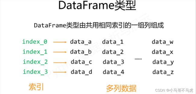
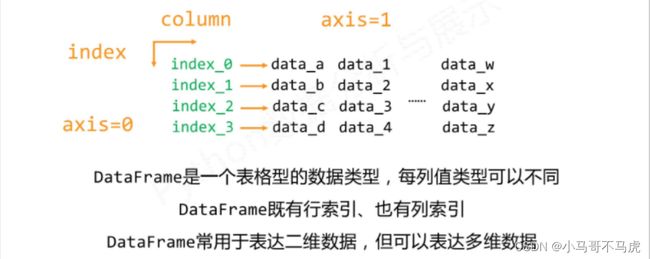
1.DataFrame类型的创建 

·二维ndarray对象

·由一维ndarray，列表，字典，元组或Series构成的字典

·Series类型

·其他的DataFrame类型

---

从二维ndarray对象创建：

import pandas as pd
import numpy as np
d=pd.DataFrame(np.arange(10).reshape(2,5))
print(d)
'''
  0  1  2  3  4     行索引
0  0  1  2  3  4
1  5  6  7  8  9
列
索
引
'''

---

从一维ndarray对象字典创建：

import pandas as pd
dt={'one':pd.Series([1,2,3],index=['a','b','c']),
    'two':pd.Series([9,8,7,6],index=['a','b','c','e'])}
d=pd.DataFrame(dt)
#数据根据行列索引自动补齐
c=pd.DataFrame(dt,index=['b','c','d'],columns=['two','there'])
print(d,'\n')
print(c)
'''
   one  two
a  1.0    9
b  2.0    8
c  3.0    7
e  NaN    6 

   two there
b  8.0   NaN
c  7.0   NaN
d  NaN   NaN
'''

---

从列表类型的字典创建：

import pandas as pd
d1={'one':[1,2,3,4],'two':[9,8,7,5]}
d=pd.DataFrame(d1,index=['a','b','c','d'])
print(d)
'''
  one  two
a    1    9
b    2    8
c    3    7
d    4    5
'''

---

四.Pandas库的数据类型操作

通过增加或重排及删除来改变Series和DataFrame对象

1.重新索引

.reindex()能够改变或重排Series和DataFrame的索引

格式：

.reindex(index=None,columns=None,fill_value,limit,copy)

·index，columns：新的行列自定义索引

·fill_value：重新索引中用于填充缺失位置的值

·method：填充方法，ffill当前值向前填充，bfill向后填充

·limit：最大填充数

·copy：默认为True，生成新的对象，False时，新旧相同不复制

代码实例：

 

import pandas as pd

d1={'城市':['北京','上海','广州','深圳','沈阳'],
    '环比':[101.5,101.2,101.6,101.1,101.4],
    '同比':[123.7,133.2,124.2,142.0,122.2],
    '定基':[152.0,147.3,132.2,155.3,132.9],}
d=pd.DataFrame(d1,index=['c1','c2','c3','c4','c5'])
e=d.reindex(index=['c5','c4','c3','c2','c1'])
c=d.reindex(columns=['城市','同比','环比','定基'])
new=d.columns.insert(4,'新增')  #增加索引
f=d.reindex(columns=new,fill_value=200)
print('原数据:\n',d)
print('index定义行:\n',e)
print('columns定义列:\n',c)
print('增加索引自动填充:\n',f)
'''
原数据:
     城市     环比     同比     定基
c1  北京  101.5  123.7  152.0
c2  上海  101.2  133.2  147.3
c3  广州  101.6  124.2  132.2
c4  深圳  101.1  142.0  155.3
c5  沈阳  101.4  122.2  132.9
index定义行:
     城市     环比     同比     定基
c5  沈阳  101.4  122.2  132.9
c4  深圳  101.1  142.0  155.3
c3  广州  101.6  124.2  132.2
c2  上海  101.2  133.2  147.3
c1  北京  101.5  123.7  152.0
columns定义列:
     城市     同比     环比     定基
c1  北京  123.7  101.5  152.0
c2  上海  133.2  101.2  147.3
c3  广州  124.2  101.6  132.2
c4  深圳  142.0  101.1  155.3
c5  沈阳  122.2  101.4  132.9
增加索引自动填充:
     城市     环比     同比     定基   新增
c1  北京  101.5  123.7  152.0  200
c2  上海  101.2  133.2  147.3  200
c3  广州  101.6  124.2  132.2  200
c4  深圳  101.1  142.0  155.3  200
c5  沈阳  101.4  122.2  132.9  200
'''

---

2.索引类型

索引类常用方法

方法	说明
.append(idx)	连接另一个Index对象，产生新的Index对象
.diff(idx)	计算差集，产生新的Index对象
.intersection(idx)	计算交集
.union(idx)	计算并集
.delete(loc)	删除loc位置处的元素
.insert(loc,e)	在loc位置增加一个元素e

import pandas as pd

d1={'城市':['北京','上海','广州','深圳','沈阳'],
    '环比':[101.5,101.2,101.6,101.1,101.4],
    '同比':[123.7,133.2,124.2,142.0,122.2],
    '定基':[152.0,147.3,132.2,155.3,132.9],}
d=pd.DataFrame(d1,index=['c1','c2','c3','c4','c5'])
nc=d.columns.delete(2)  #删除
ni=d.index.insert(5,'c0')
nd=d.reindex(index=ni,method='ffill')
print('原数据:\n',d)
print('删除第三个:\n',nc)
print('增加c0:\n',ni)
print('操作后:\n',nd)
'''
原数据:
     城市     环比     同比     定基
c1  北京  101.5  123.7  152.0
c2  上海  101.2  133.2  147.3
c3  广州  101.6  124.2  132.2
c4  深圳  101.1  142.0  155.3
c5  沈阳  101.4  122.2  132.9
删除第三个:
 Index(['城市', '环比', '定基'], dtype='object')
增加c0:
 Index(['c1', 'c2', 'c3', 'c4', 'c5', 'c0'], dtype='object')
操作后:
      城市     环比     同比     定基
c1   北京  101.5  123.7  152.0
c2   上海  101.2  133.2  147.3
c3   广州  101.6  124.2  132.2
c4   深圳  101.1  142.0  155.3
c5   沈阳  101.4  122.2  132.9
c0  NaN    NaN    NaN    NaN
'''

---

四.Pandas库的数据类型运算

算术运算根据行列索引补齐后运算，运算默认产生浮点数，补齐时缺项填充NaN

1.符号形式的运算：+ - * /

import pandas as pd
import numpy as np
a=pd.DataFrame(np.arange(12).reshape(3,4))
b=pd.DataFrame(np.arange(20).reshape(4,5))
print('加运算:')
print(a+b)
print('乘运算:\n',a*b)
print('减运算:\n',a-b)
print('除运算:\n',a/b)
'''
加运算:
      0     1     2     3   4
0   0.0   2.0   4.0   6.0 NaN
1   9.0  11.0  13.0  15.0 NaN
2  18.0  20.0  22.0  24.0 NaN
3   NaN   NaN   NaN   NaN NaN
乘运算:
       0     1      2      3   4
0   0.0   1.0    4.0    9.0 NaN
1  20.0  30.0   42.0   56.0 NaN
2  80.0  99.0  120.0  143.0 NaN
3   NaN   NaN    NaN    NaN NaN
减运算:
      0    1    2    3   4
0  0.0  0.0  0.0  0.0 NaN
1 -1.0 -1.0 -1.0 -1.0 NaN
2 -2.0 -2.0 -2.0 -2.0 NaN
3  NaN  NaN  NaN  NaN NaN
除运算:
      0         1         2         3   4
0  NaN  1.000000  1.000000  1.000000 NaN
1  0.8  0.833333  0.857143  0.875000 NaN
2  0.8  0.818182  0.833333  0.846154 NaN
3  NaN       NaN       NaN       NaN NaN
'''

---

2.方法形式的运算

方法	说明
.add(d,**argws)	加法运算
.sub(d,**argws)	减运算
.mul(d,**argws)	乘法运算
.div(d,**argws)	除法运算

import pandas as pd
import numpy as np
a=pd.DataFrame(np.arange(12).reshape(3,4))
b=pd.DataFrame(np.arange(20).reshape(4,5))
print('减运算:\n',b.sub(a,axis=0))    #fill_value用来替代NaN
print('加运算:\n',b.add(a,fill_value=100))
print('乘运算\n:',b.mul(a,fill_value=0))
'''
减运算:
      0    1    2    3   4
0  0.0  0.0  0.0  0.0 NaN
1  1.0  1.0  1.0  1.0 NaN
2  2.0  2.0  2.0  2.0 NaN
3  NaN  NaN  NaN  NaN NaN
加运算:
        0      1      2      3      4
0    0.0    2.0    4.0    6.0  104.0
1    9.0   11.0   13.0   15.0  109.0
2   18.0   20.0   22.0   24.0  114.0
3  115.0  116.0  117.0  118.0  119.0
乘运算
:       0     1      2      3    4
0   0.0   1.0    4.0    9.0  0.0
1  20.0  30.0   42.0   56.0  0.0
2  80.0  99.0  120.0  143.0  0.0
3   0.0   0.0    0.0    0.0  0.0
'''

---

3.比较运算

比较运算只能比较相同索引的元素，采用< > >= <= == !=等符号进行运算产生布尔对象

 

 

---